本节内容,来自Modern Rendering with Metal
关联阅读:
In the first part of the session, I will go over some of the more advanced rendering techniques that you can use in your apps today.
Then my colleague, Srinivas Dasari, will talk to you about moving your CPU render loop to a more GPU-driven pipeline.
We'll end the session by showing you how we can use our new GPU families to easily write cross spectrum code.
Advanced Rendering Techniques
Whether you're starting from scratch or you want to improve your existing Metal app, or you have an amazing rendering engine that you want to move onto the Metal platform, we'll show you how you can make the best use of the available hardware with the rendering technique that fits your needs.
We'll start by taking a look at some of the range of rendering techniques that are used by games and apps today.
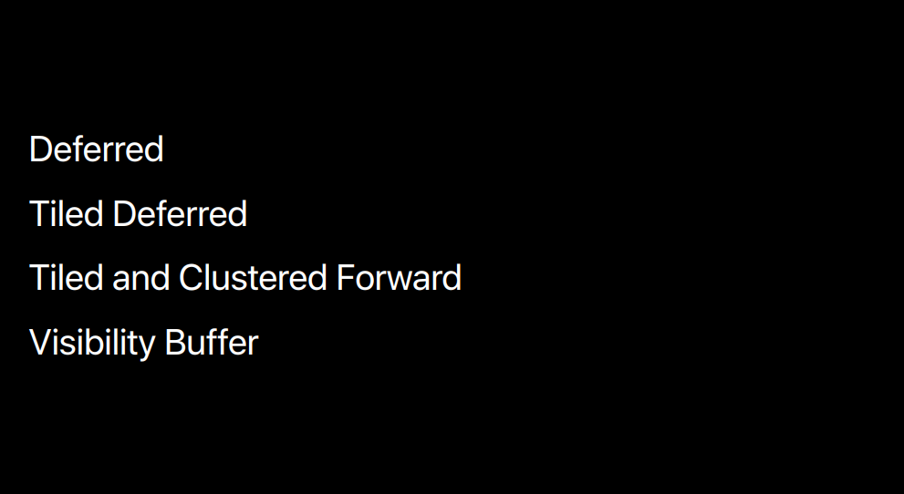
We'll start with basic deferred rendering.
This is the most commonly used rendering technique used by games and graphical apps on all platforms.
We'll discuss the classic two-pass setup.
We will show you how to implement this in Metal and how to optimize this for the iOS platform.
We'll then move on to tiled deferred, which extends the lighting pass of deferred rendering and is perfect if your art direction requires you to have complex lighting setups.
We'll then take a look at forward rendering.
That's a really good alternative for the Metal apps that require complex materials, anti-aliasing, transparency, or special performance considerations.
Our last technique we're going to talk about is visibility buffer rendering, which defers the geometry logic all the way back to the lighting pass and now in Metal 3, is easier to implement than ever.
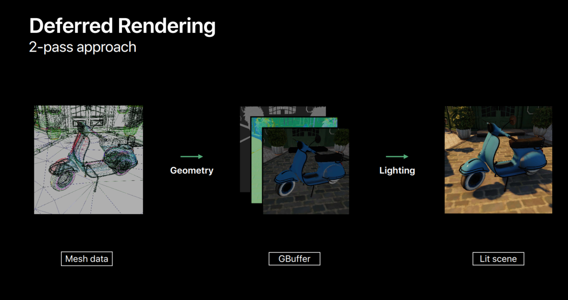
But before we get there, let's start with deferred rendering.
Deferred rendering splits the rendering of your scene up into two passes.
There's the geometry pass, where you basically render your entire scene into an intermediate geometry, or g-buffer.
And the textures in this buffer, all the normal, the albedo, the roughness, and any kind of surface or material property that you need in your writing model or your postdressing pipeline.
Then in the second pass, the lighting pass renders the light volumes of your scene and builds up the final lit scene in accumulation texture.
The deferred light shaders were bind all the textures in your G-buffer to calculate their contribution to the final lit surface color.
So, let's define the data flow of this technique and then move onto a Metal implementation.
So, here we have our two render passes, and we'll be running these two consecutively on the GPU.
In our geometry pass, we need to write out depth.
The depth is used to do depth calling during your geometry pass, but it's also used to calculate the pixel location and world space for your lighting pass.
And we also output our G-buffer textures.
In our example here, we'll use normal, albedo, and roughness textures.
Then in our second pass, the lighting pass, we read back the G-buffer textures and then we draw light volumes and accumulate them in our output texture.
So, let's see how we can construct this data flow in Metal.
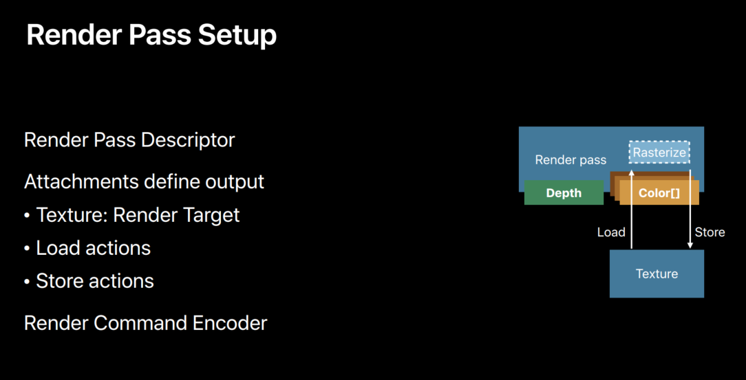
To set up a render pass in Metal, you have to start with a Render Pass descriptor.
The most important part of a Render Pass descriptor are its outputs.
In Metal, these are defined with attachments.
Every Render Pass can have single depth attachments and multiple color attachments.
For every attachment, we have to define the texture which points to the data that stores our attachment data.
We have to define our load action which shows us how to load the existing data from the texture and the store action is how to store the results of your rendering back into the texture.
When you've defined these properties of all your attachments, you can then create your Render command encoder that you can then use to finally draw your objection to your Render Pass.
Now, let's see how we build this in Metal, starting with our setup code.
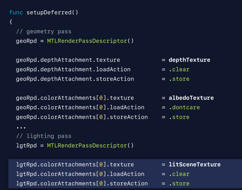
So, here we have our setup function.
We'll start by creating a Render Pass descriptor.
And now we just start filling in all these attachments.
So, we'll start with the depth attachment.
And since we're using the depth attachment to do our depth calling, we need to make sure it's clear before we start rendering our scene.
So, we set our load action to clear.
Of course we want to store depth for the second pass.
So, we set R, store action to store.
Now, we move onto our color attachments.
The color attachments, we need one for every texture in our G-buffer.
And because all these textures are going to be handled kind of the same way, we'll just show you the albedo.
Because we're probably going to be using like a skybox or a background during rendering, so, we're sure that we're going to be overriding every pixel in our frame, every frame.
Which means we don't really care about any previous values in our G-buffer textures. So, we can set our load action to dontcare.
Of course, we want to store the results of our G-buffer, so we set our store action to store.
Now we can start with our lighting pass descriptor.
We create another descriptor object, and then we defined attachment for accumulation buffer.
Since we're accumulating data, we need to clear it before starting so we put our load action to clear.
And of course we want to save our final image, so our store action's going to be store.
Now, let's look at render loop while we're using these Render Passes to actually draw our scene.
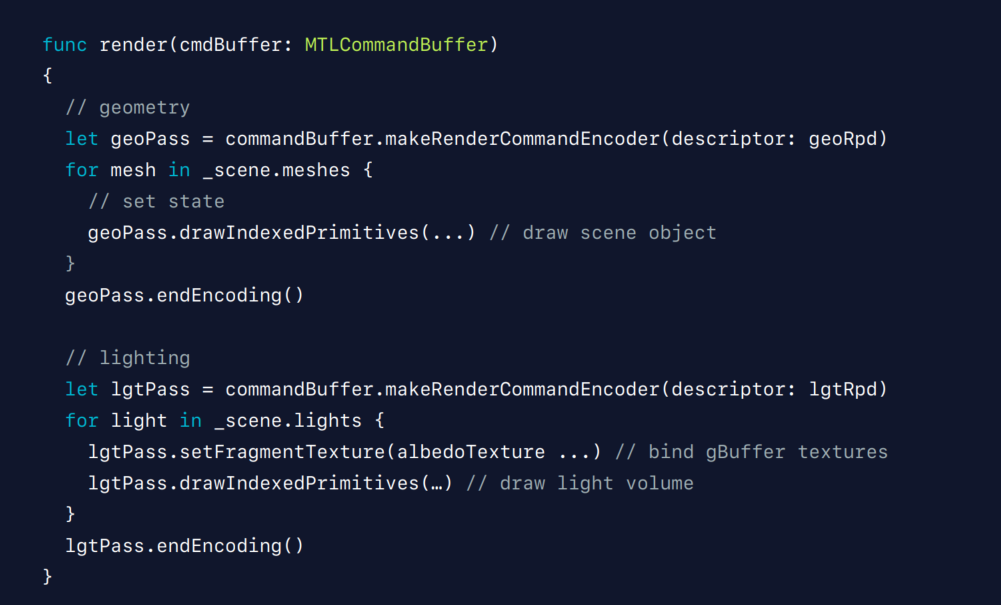
So, we'll start again with our geometry pass.
We create our Render command encoder using our descriptor.
And then we start just iterating over all the measures in our scene.
This is a very simple way of rendering your scene.
And my colleague, Srinivas, will show you in the second part of this session how you can move this basic CPU render loop into a more GPU-driven pipeline with all kinds of calling and LOD selection.
Okay, so now we've encoded our entire geometry pass, and we move on to our lighting pass.
We create another render command encoder.
And we now we start iterating over all the lights for our lighting pass.
And every light, every deferred light shader will bind those textures from the G-buffer to calculate its final light colors.
Well, this two-pass system works perfectly fine on macOS and iOS across all platforms.
It's a really good fit for all types of hardware.
But there are some things that we can do to further optimize our implementation on iOS.
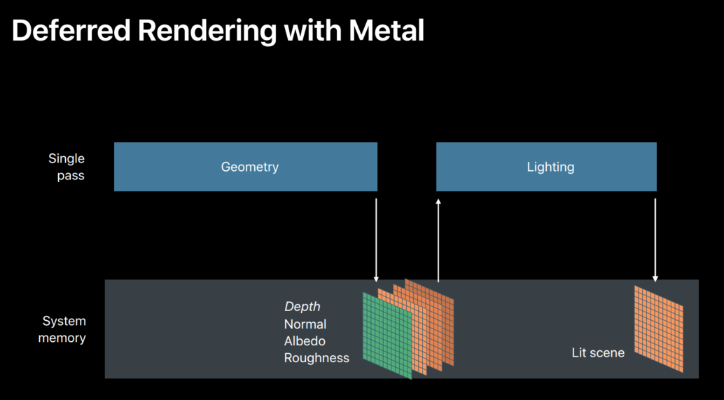
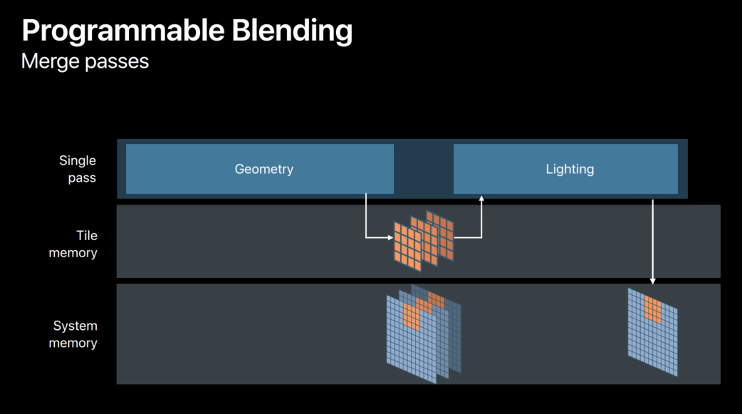
So, let's step back from the code back into our overview.
You can see there's this big buffer between our two render passes.
The geometry pass is storing all its data into these G-buffer textures.
And then the lighting pass is bringing them all back.
And if we're having multiple lights shining on a single pixel, we're doing this readback multiple times.
Using a technique called programmable blending in Metal, we can get rid of this intermediate load store into device memory by leveraging the taut architecture of iOS devices.
So, how do we take advantage of this technique? Well, to enable programmable blending, we merge the geometry and the lighting pass, and create a single render encoder for both Geometry and light rules.
So, due to the nature of iOS architecture, the attachments are kept resident in tile memory for the entire duration of our encoder.
This means we can't only write to our attachments but we can actually read them back.
We can read back the values of the same pixel we're writing, and this is exactly what we want.
We want, when we're calculating the light in our lighting pass, we want to retrieve the written G-buffer attachments of the same pixel.
So, let's see how this will affect our light shaders.
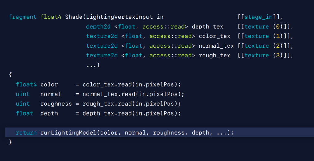
So, here we have a light fragment shader from our lighting pass.
And as you might know, you just start by binding all the textures that you need to get your G-buffer data.
And then you have to actually read all these textures across all your G-buffer textures to get all the material and surface information.
Only then can you push this into your lighting model to get your final vid color.
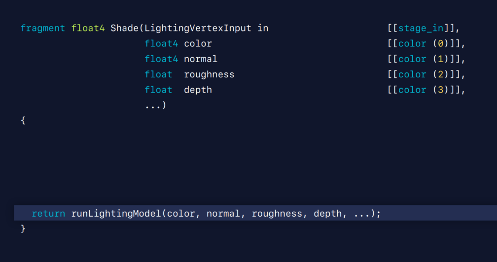
Now, let's see what happens if we use programmable blending.
Instead of binding all the textures, we simply bind all the color attachments.
And now we can directly use these values in our lighting model.
As you can see, we've created a new linear depth color attachment for our G-buffer and this is because when you're using programmable blending, you cannot access the depth attachments.
So, now that we're no longer binding or sampling any textures, let's see how we can use this to further optimize our memory layout.
When using programmable blending, we're no longer writing or reading from the G-buffer textures.
So, we can put the store action of our color attachments to dontcare.
So, this solves our bandwith problem, but we still have these Metal texture objects taking up space in our device.
And we need to tell Metal that we no longer need any physical memory for our G-buffer textures.
And we do this by setting the storage mode of the texture to memoryless and we tell Metal that we're no longer going to basically be performing any store actions on it, so we don't need to actually allocate the memory.
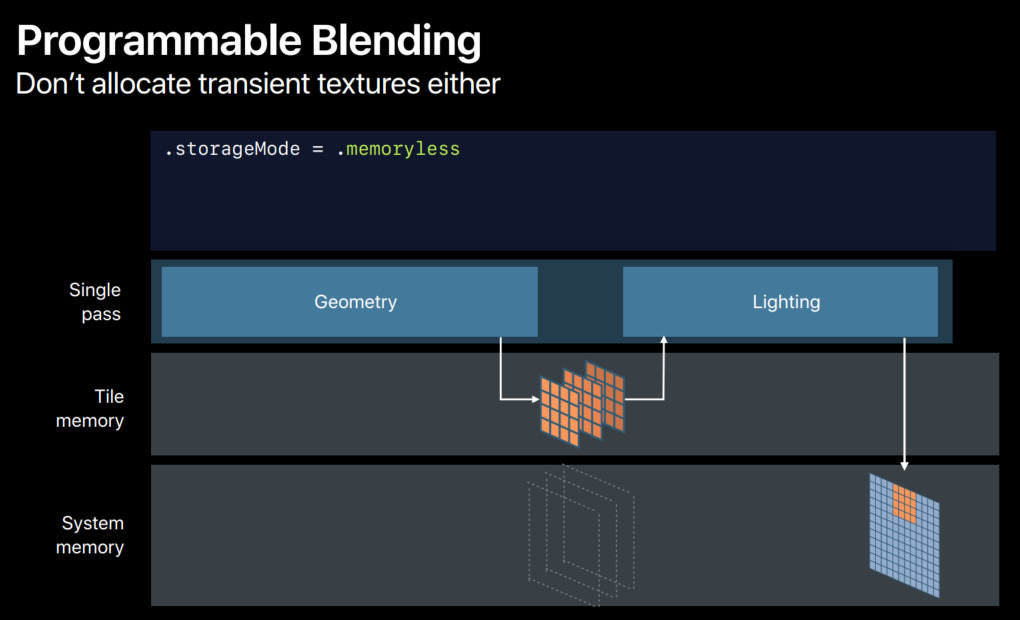
With these steps, we've now end up with an iOS implementation that has all the benefits but without any of the memory or bandwith overhead of a G-buffer.
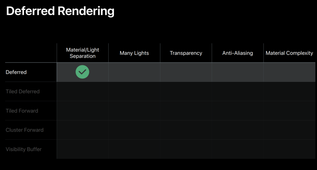
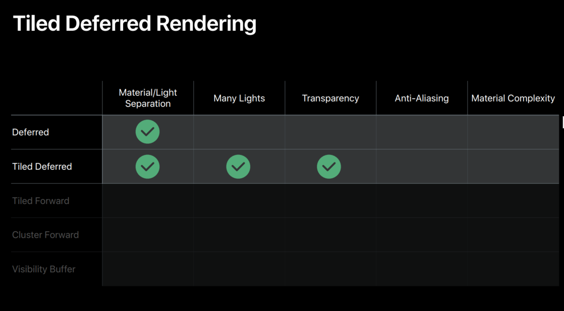
Before I move on to tile deferred, let's summarize.
The separation of the geometry and lighting pass makes this a very versatile technique.
It handles both complex geometry and lighting very well.
And a G-buffer can be used to facilitate a really deep postprocessing pipeline.
And an entire pipeline can be put in line using this programmable blending method.
On macOS, you still have to deal with a G-buffer, memory, and bandwith overhead.
So, now let's move on to tiled lighting solution, which is ideal for those of you who want to render maximum amount of light but you still want to reduce your light pass overhead.
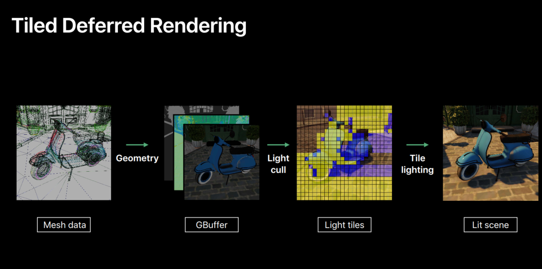
The tiled deferred rendering technique tries to solve the performance issues of rendering large amounts of lights.
In classic deferred, we render every light separately, and this causes a lot of the G-buffer overhead for overlapping lights.
Tile deferred rendering extends the lighting with an additional compute prepass that allows our shading to happen not on a per light level but on a per tile level.
The prepass first divides our screen into a 2D grid of lighting tiles and generates a light list per tile.
Then in a second step, the lighting step itself, these lights are then used to efficiently light the tile using a single light fragment shader, but it's ranging over the lights in the light list.
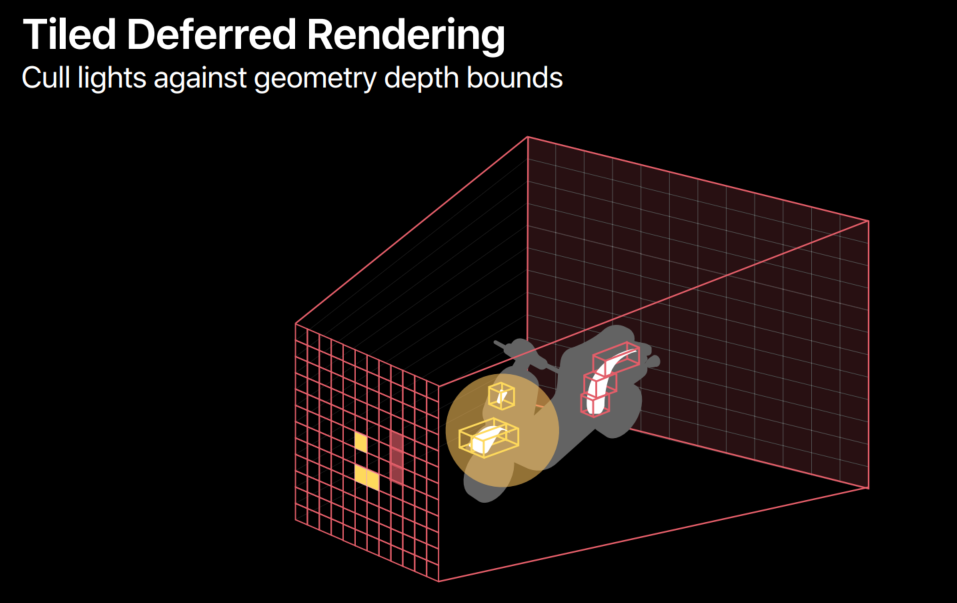
Before we dive into the implementation details, let's take a quick look at how these light lists are being generated.
Well, we first split up our view frustums into these small subfrustums, one for each tile.
Then we use our compute shader to further fit down the subfrustums using the location of our tile, but also the depth bounds of the tile.
And we can do this because we've already ran the geometry pass.
So, the depth buffer is already populated.
So, when we fitted down these subfrustums, we can then just test all the frustums against the light volumes and add any intersections to our light list.
This entire process can be done in parallel across al the tiles and is a perfect fit for a compute kernel.
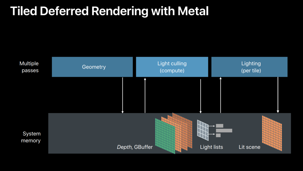
So, how do we integrate this into our deferred pipeline we showed before? Well, before we had this two-pass deferred setup.
And now we've added this compute pass to the middle of it.
And that will create in the light list for us and we need to store these light lists in a light list buffer to be stored in device memory.
So, again, this solution works fine on all platforms and it simply requires us to create additional compute and to move our lighting logic from a single light per shader to an iterative loop in our lighting shader.
Just like with the previous rendering, we can now take advantage of the hardware tiling on iOS to further optimize this.
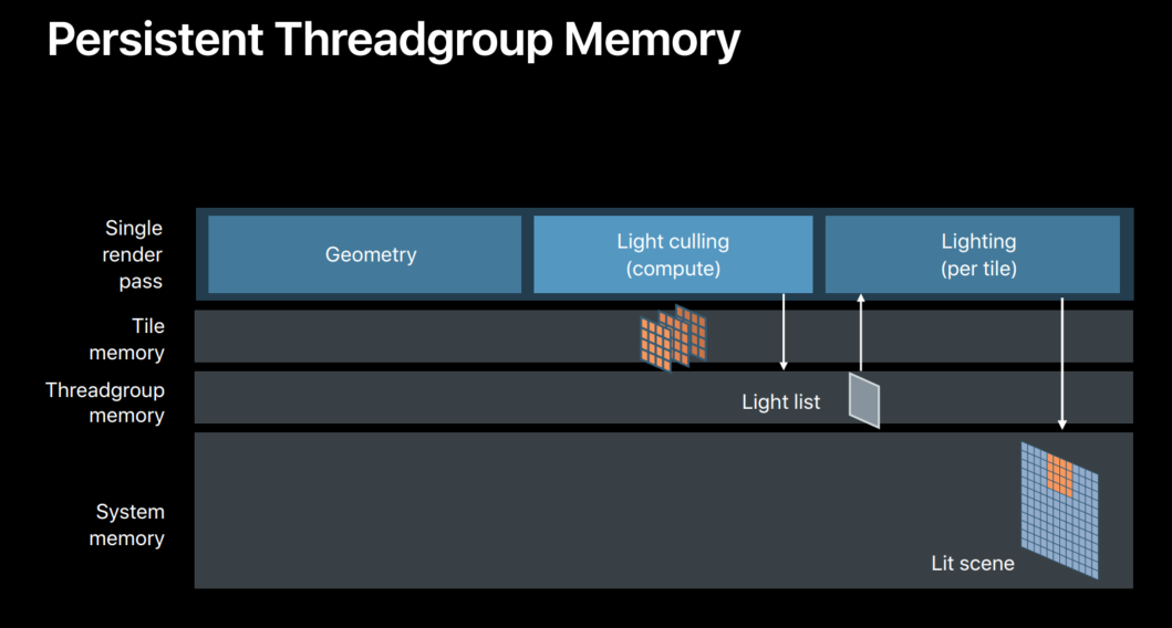
So, let's take a look of how this fits in our single encoder iOS implementation.
So, here we have our single pass solution we showed before, and we need to get this computer in there, but we need to stay within the single render command encoder to use the programmable blending.
Metal provides an efficient way of using tile-based hardware architecture to render compute work on each tile that we're restorizing.
For this purpose on iOS, the render command encoder can encode tiler shader pipelines to run the compute functions.
And this is a perfect fit for outside lighting because now we can take our lighting tile concept and map that directly on our hardware tiles.
So, now that our light calling prepass can be run directly on our hardware tile, we can use a second Metal feature called persistent thread group memory to store the resulting light list alongside our attachments in tile memory.
Which then can be read back, similarly to the attachments but all the draws in the render command encoder.
Which in our case is going to be our per light draws.
We now move our lighting back end to execute in line with our graphics and completely within tile memory.
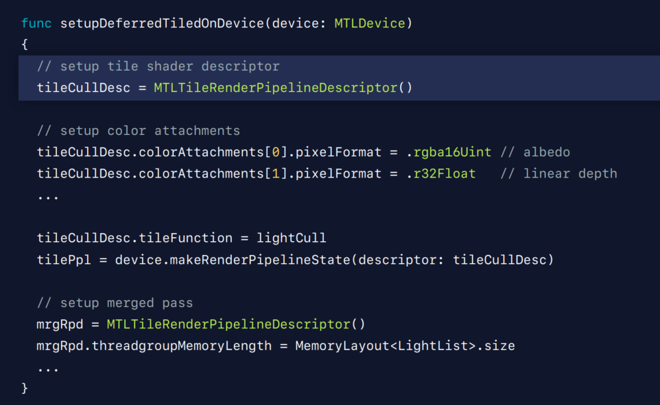
So, what does this look like in Metal? Let's move back to our setup code.
Creating a tile shader is very similar to setting up a normal render pipeline state.
We create our descriptor.
We set up all our color attachments.
We then set up our compute function we want to execute.
And we simply create our pipeline state.
Because we are using the precision thread group memory, we need to reserve a little bit of memory in our tile.
So, we go back to our render pass descriptor and then we simply reserve just enough data to store our light list.
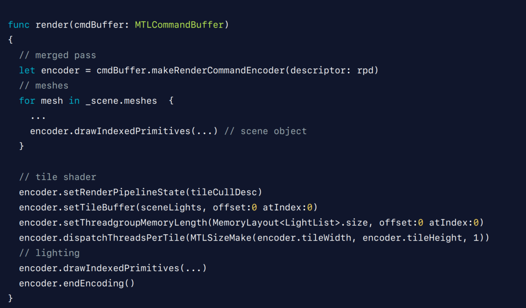
Now, let's move on to the render loop to see the dispatch size of these things.
So, our render loop starts this time with a single render command encoder.
And we again loop over all the meshes in our scene.
And then instead of directly going to the lighting pass, we first have to execute our tile shader.
So, we set up our pipeline state, we set a buffer that holds all the lights within our scene, and then we bind the thread group memory buffer into our tile memory.
And then we simply dispatch our tile shader.
Now that we've executed our tile shader, the thread group memory we hold, the light list, we can then use in the lighting draw where we can have every pixel having access to its tiles light list using the persistent thread group memory and now very efficiently can shade its pixels.
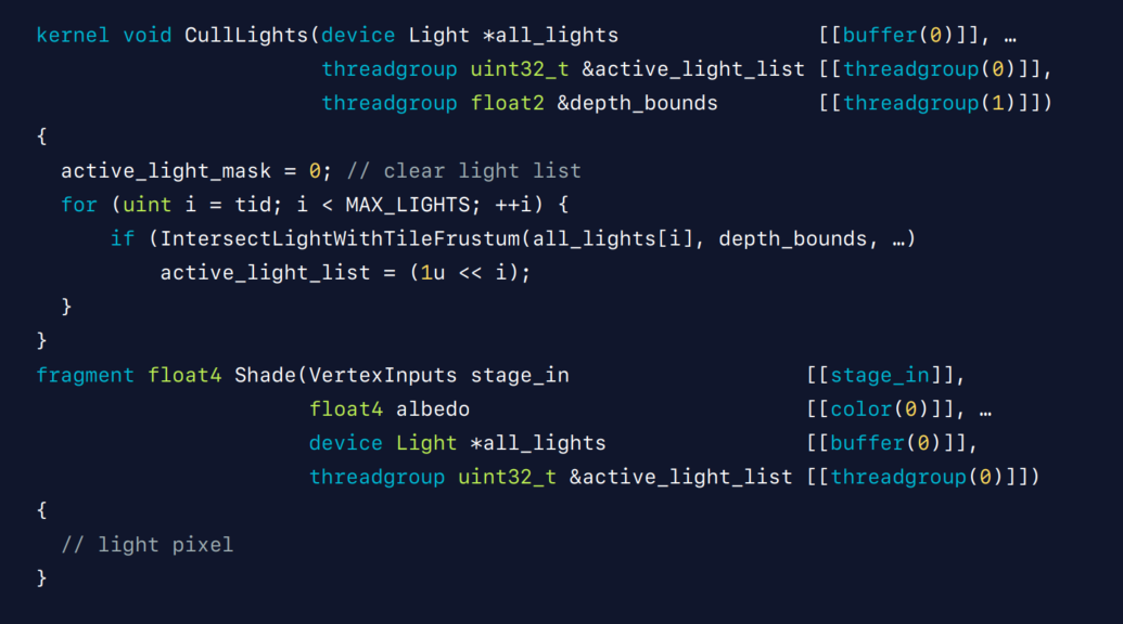
Now finally, after all is set up, let's see what this looks like in our shaders.
So, here we have two shaders.
The top one is the tile shader.
It's binding the output light list into a persistent thread group memory buffer.
Then it basically loops over all the lights in some way and it outputs the light mask into the persistent thread group memory, which can then be read back by the second shader, our actual lighting shader.
And then it's right over all the visible lights within its tile and shade our pixels.
Now that we've seen all these key points of implementing the tiled lighting technique for our tile deferred technique, let's see how we can use this principle to extend our renderer to frame additional forward pass efficiently.
Because we've set up our light list in a persistent thread group memory, we can use the same data to accelerate an effective tiled forward pass.
Whenever we're shading our forward geometry in our forward pass, we can simply use that same persistent thread group memory to read our tile light list and use the same light loop that we've been using in our deferred lighting to very efficiently shade our forward pixels.
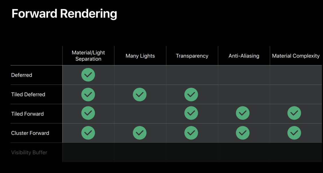
This forward pass really rounds out the capabilities and allows for transparency, special effects, and other complex shading that would normally not be possible with just deferred.
However, there's always some limitations to a deferred pipeline.
Anti-aliasing.
Complex material expressions are still a problem due to the intermediate G-buffer representation.
What we have seen is using this tile technique we can very efficiently accelerate forward rendering using the tiled lighting technique.
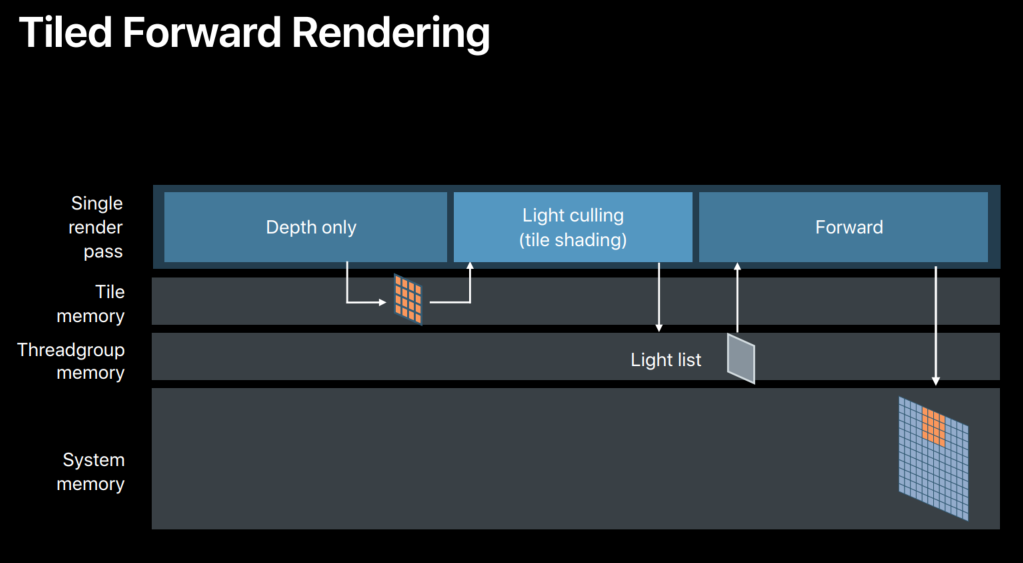
So, let's take a step back and focus purely on that forward pass, because alongside with tiled lighting, this becomes a viable solution in its own right.
To create a forward only renderer, we simply remove the deferred geometry and lighting pass. However, our light calling technique needs that depth to fit its subfrustums.
So, we need to replace our geometry pass with a depth prepass to fill this depth buffer.
And if your engine already has such a depth prepass, this is the perfect solution for you.
So, if you have one beat for overdraw, optimization, inclusion calling, or self-blending, this solution will fit your needs.
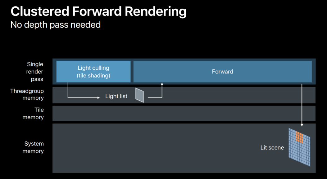
However, on iOS hardware, such a pass is often unnecessary.
And for those cases, a different lighting solution, called clustered lighting, might be a better fit for you.
This clustered solution has a different way of creating the light lists that does not require any depth.
Because for clustered lights, we don't create any depth bounds for our tiles but we simply subdivide the frustums along the depth axis.
And we then emit a 3D light list map instead of a 2D light map.
It might not be as efficient as our fitted subfrustums from our tiled lighting but it will give us a measurably improved performance on lighting, where every pixel is only shaded by a local light list.
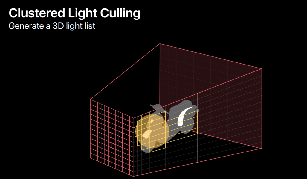
Using clustered calling combined with tile shading and persistent thread group memory, this gives us very optimized forward rendering.
We've seen now a few of the most popular pipelines and how to implement them on Metal.
Now we're going to look at the visibility buffer rendering technique that tackles the G-buffer overhead in a different way, making it more suitable for old hardware that does not support hardware tiling.
Let's go all the way back to our deferred renderer.
So, most of the optimization we've shown so far only work on the iOS architecture.
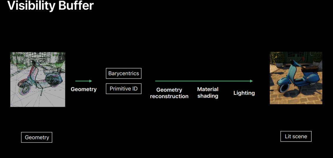
The visibility buffer technique tries to minimize the intermediate buffer bottleneck in another way, namely by storing the absolute minimum amount of data in that buffer.
Instead of storing all the surface and material properties per pixel, we only store a primitive identifier and barycentric coordinates.
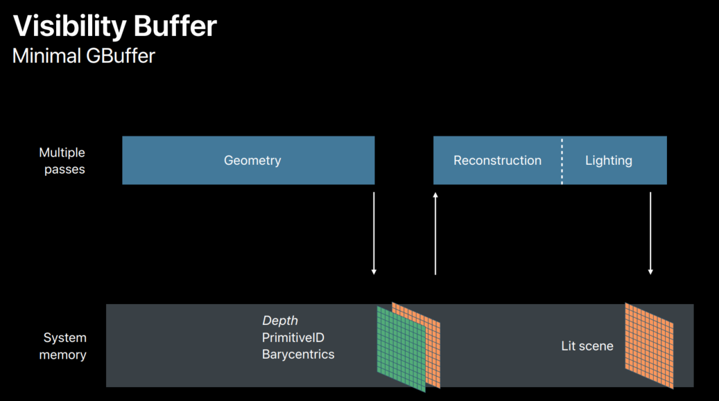
This data cannot be used directly to shade your entire scene, but it can be used to reconstruct and interpolate the original geometry, and then locally run your entire material logic within the lighting shaders.
Since this reconstruction step is very costly, this works very well with the tiled lighting technique because that guarantees we're only going to use reconstruction step once per pixel.
When we're implementing this technique, the biggest problem is usually how to create these primitive indices and how to create these barycentric coordinates without a lot of additional processing.
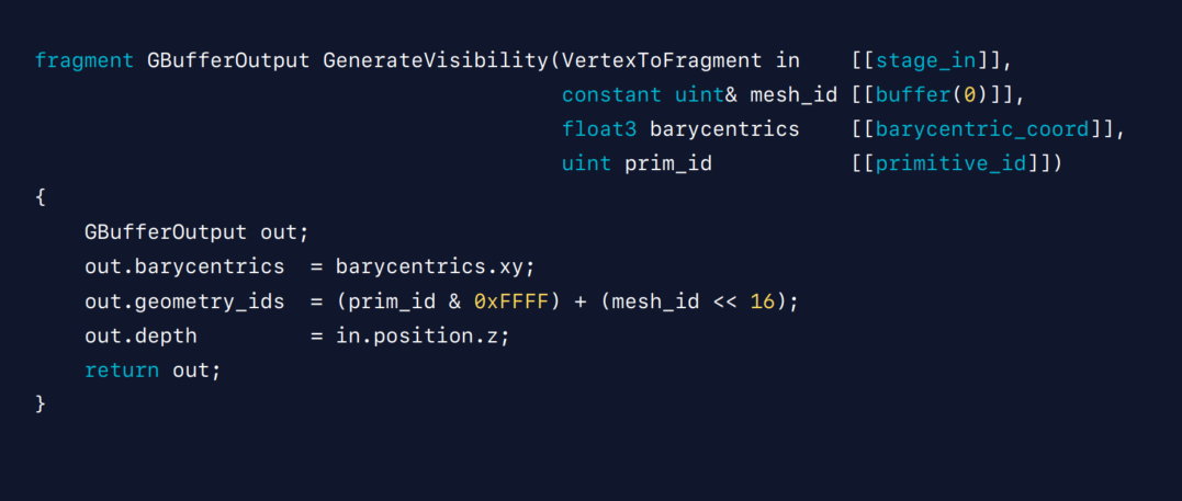
We're now happy to tell you that in Metal 3, you can now retrieve the index of your current primitive and the barycentric coordinate of your current pixel within your fragment shader using these two new attributes.
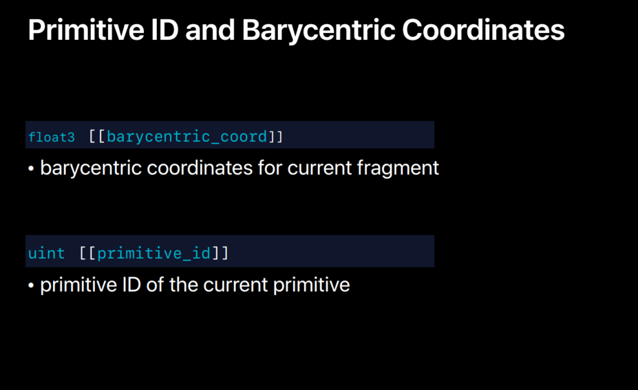
The resulting geometry shader is now extremely simple, making your geometry pass faster than ever and making it easier to implement than ever using Metal 3.
We've now gone over all these different options that you can use to render your scene in Metal.
Now let's look at a little demo that showcases some of these rendering techniques.
So, here we have our test scene, which has some rather complex geometry and setup PBR materials and array of different material shaders.
We can use deferred or tile deferred, or even forward to render this scene on any of your devices.
Let's start with the normal deferred renderer.
The deferred renderer has two passes, as we've shown before.
And the first pass is now rendering everything through these intermediate G-buffers.
Let's look at some of those G-buffer textures now.
So, here we have the albedo.
We have the normal.
And we have the roughness texture of our G-buffer.
If you have temporal and aliasing, or more complex lighting models, you'll probably need to store more in the G-buffer.
The scene we're seeing right now is being lit by that second lighting pass.
So, let's go to a night scene to visualize our lights a little bit better.
Now, in this scene, to get it lit up like this, we need to render a lot of lights, which we are visualizing here.
In normal deferred, we should be rendering all of these lights one at a time, which is very inefficient.
And you can see there's lots of overlap between the different lights.
So, let's move on to a tile deferred lighting.
So, here we have the same scene rendering using tile deferred renderer.
What we want to show here was all the possible visualizations we had for how the different tiles, show you the amount of lights that are being rendered in each of these different tiles.
And you can see that it really makes a difference in using these tiled subdivisions, relative to just lighting all the pixels with all the lights at once.
Now, we've shown you some of these possible rendering techniques that you can use to render your scene.
GPU-Driven Pipelines
And now my colleague Srinivas will show you in the next part how you can turn your CPU heavy render loop into a GPU-driven pipeline.
With Metal 2, we introduced the GPU-driven pipelines which consist of augment buffers and indirect command buffers with which you can now move your CPU-based rendering operations to the GPU.
My colleague just showed you how to implement various advanced rendering techniques with Metal.
In this talk, I'm going to show you how to move your entire CPU-based render loop to the GPU.
Now, this will not only make your render loop more efficient but it allows you to free up your CPU for any other processing that you may want to do, like complex physics simulations REI.
Now, before diving into details, let's first see what operations are usually performed in a render loop.
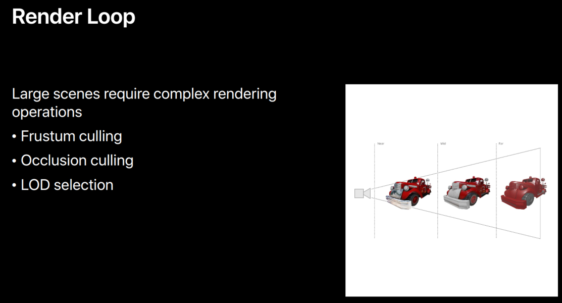
Now, large scenes require complex rendering operations.
So, usually you do a series of operations to efficiently render the scene.
So, the first thing that you do is frustum culling, where you remove the objects that fall outside the view frustum.
We only show draw calls for those.
Next, occlusion culling.
Here you eliminate the objects that are occluded by other, bigger objects.
Another thing that usually done is level of detail selection, where you select between a range of levels of details of the model based on its distance to the camera.
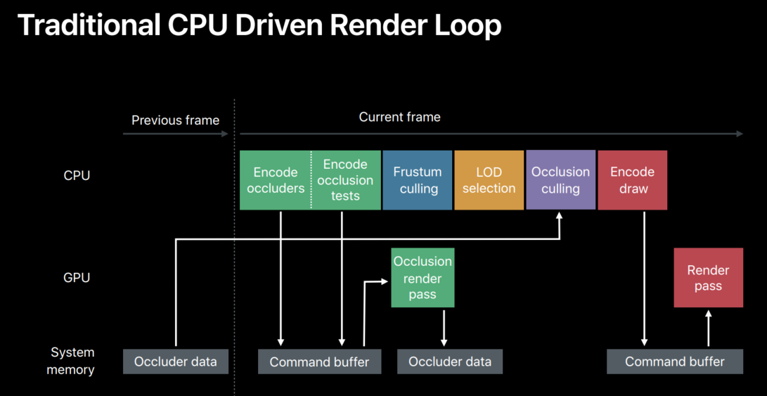
So, your CPU-based render loop with all these operations typically looks like this.
Basically, you first encode your occluded and occlusion test into your command buffer and you execute it in a render pass on the GPU to generate occlude data for the next frame.
Next, you do frustum culling, eliminate the objects that are outside the view frustum.
And LOD selection to pick a level of detail of the model and occlusion culling, to eliminate the objects that are occluded other, bigger objects.
So finally, you enclosed the pass for visible objects and execute it in a render pass to generate your scene.
Now, this works fine but there are a couple of inefficiencies here.
First let's take occlusion culling.
Now, to do occlusion culling, you need occlude data for the current frame.
But because you don't want to introduce any synchronizations in the current frame, you usually rely on the previous frame's occluder data, which is usually obtained at a lower resolution.
So, it can be approximate.
It can lead to false occlusion.
And so you probably have to take some corrective steps in your gains.
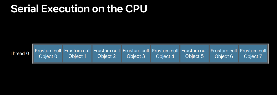
And second, there are operations here that are highly paralyzable.
For example, frustum culling.
On a single CPU thread it looks like this, where you'll be doing frustum culling of each object, one after the other.
Now, you can definitely distribute this processing across multiple CPU threads but there are only a few CPU threads available.
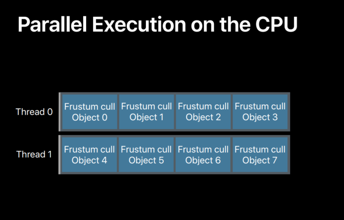
And if you include all other operations that you want to perform per object, you'll probably be doing something like this.
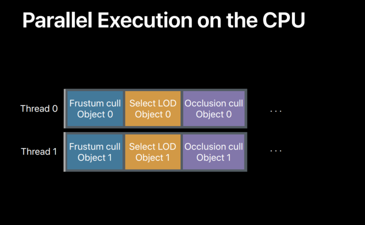
But are these operations highly paralyzable? So, if you have more threads, you can pretty much process all the scenes, all the objects in our scene in parallel.
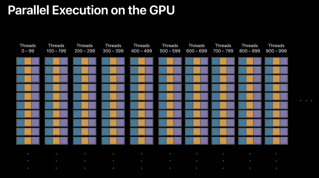
But typically, there are thousands of objects in a scene and so to paralyze all of them, you need thousands of threads.
So, the perfect choice for these operations is the GPU.
Now, GPU is a massively parallel processor with thousands of threads available to schedule operations on.
So, it is possible to assign an object to a dedicated thread and perform all the operations that we want to perform on that object.
And with thousands of threads, you can process thousands of objects in parallel.
So, your render loop is going to be more efficient if you move it from CPU to GPU and as I mentioned before, it will also be freeing up your CPU for any other processing you want to do.
So, how do you move all these operations to the GPU.
You can do it with a combination of compute and render passes on the GPU so that we can drive the entire render loop on the GPU without any CPU involvement.
This idea, I mean, this is what we need.
The entire render loop here is on the GPU.
It's completely GPU driven.
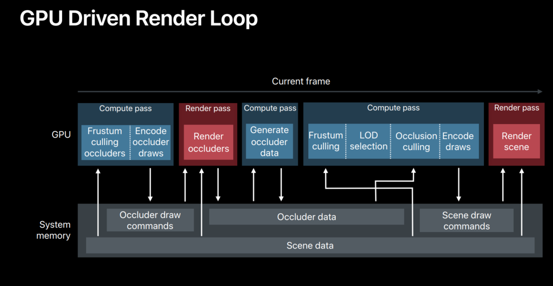
Now, let's go through these passes to see how this GPU-driven render loop really works.
Now, we need occluder data for occlusion culling.
So first we have a compute pass that takes a scene data, does frustum culling of occluders, and enclodes commands for rendering the occluders.
Now, these encoded occluded raw commands are executed in a render pass, so we generate any required occluder data.
Now, this occluder data can be in various forms, depending on how it gets generated.
So, you may want to further process that data.
For that, we can have another compute pass.
Now in this pass, the occluder data can be converted into a form that is more suitable for occlusion culling.
We need one more compute pass for the operations we talked about.
That is, culling, a level of detail selection and for encoding of scene raw commands.
So, one thing to find out here is that occlusion culling here is no longer dependent on previous frames' data.
Required occluder data is generated for the current frame in the first two passes that we just talked about.
And also because we are generating it for the current frame, it's also more accurate.
And finally, we have another render pass that executes a scene raw commands for rendering the scene.
So, in this GPU-driven render loop, everything's happening on the GPU.
There is no CPU-GPU synchronization anywhere, no previous frame dependencies.
So, how can we build this GPU-driven pipeline? Now, it is clear that we need at least two things to be able to build this render loop on the GPU.
First, draw commands.
We need a way to encode draw commands on the GPU so that the compute pass can encode the commands for the render pass.
And the building block that Metal provides to support this is indirect command buffers.
And we also need scene data.
We should be able to access the encoded scene data on the GPU through the frame wherever it is needed.
And with this scene data, we should be able to pretty much describe the whole scene, like geometry, shared arguments, materials, etc.
So, in the building block that Metal provides to support this is argument buffers.
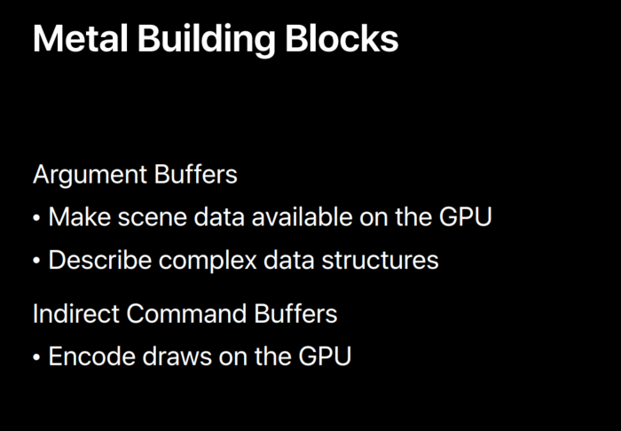
Now, let's take a more closer look at these two building blocks.
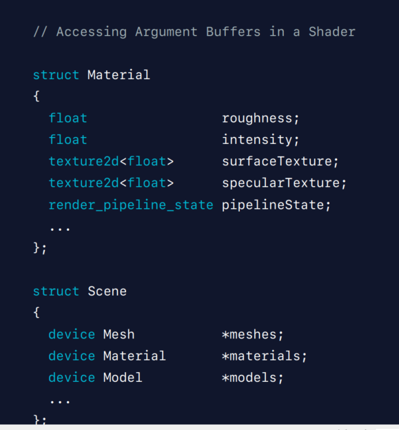
Now, argument buffers let you describe the entire scene data with complex data structures.
And they let you access the scene data anywhere in the loop.
And indirect command buffers allow you to build draw calls on the GPU and basically it supports massive parallel generation of commands on the GPU.
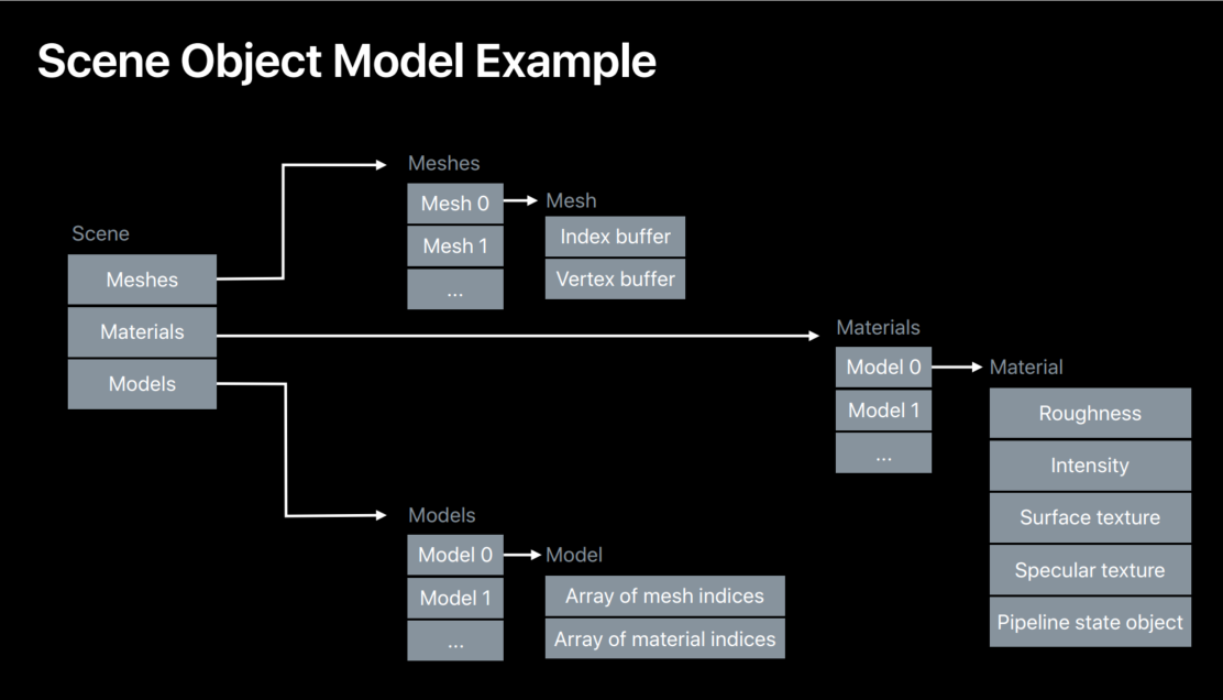
Now, let's dive into these argument buffers a little further with an example scene object model.
Now, the first thing that we need is access to scene data.
So, what does scene data really consist of? First, meshes.
Now, here is the meshes.
It is an area of mesh objects, each describing its geometry.
And Metal is an area of Metal objects each with a set of Metal properties, any textures it needs, and the pipeline steered object that describes the shadow pipeline.
And scene also consists of an area of models.
Here, each model can have an LOD so in this example, we have each model consisting of area of meshes and materials, one per LOD.
Finally, we have a scene object that relates meshes, materials, and models that are part of our scene.
So, let's see how this object model can be expressed with argument buffers.
It is a very simple 1-to-1 mapping from our object model to argument buffers.
For example, scene argument buffer here simply consists of the objects that we just described in our object model.
That is areas of meshes, materials, and models.
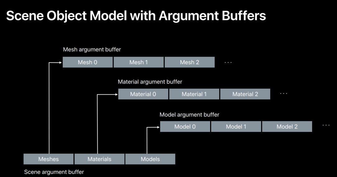
Basically, the entire scene can now be described with argument buffers.
Now, let's look at how this can be constructed and accessed in the shader.
Now, each of the argument buffers we just discussed is simply represented by a structure.
That now contains members that we have described in our object model.
Since each argument buffer is a structure that is completely flexible, you can add things like arrays, pointers, even pointers to other argument buffers.
For example, here's a Metal argument buffer.
It can contain Metal Constants any textures it needs, and of course the pipeline straight objects that describe the shadow pipeline.
So everything that is needed for a Metal is in one argument buffer.
And the scene argument buffer is just like how we described it in our object model.
So, it's just very easy to construct object models with argument buffers.
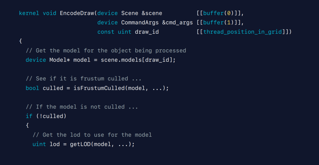
Now, let's look at how we can access these argument buffers in the sharable.
Now, this is a compute kernel that does frustum culling that we just talked about.
It encodes the draw commands for visible objects into an indirect command offer.
Each thread that executes an instance of this kernel processes one object and encodes a single draw call if it data mines that object is visible.
So, let's see how this does it.
Now, first we pass in our high-level scene argument buffer to the share.
Now, once we have access to our shader, our scene, then it is very easy to access anything else we need.
And command R here contains the reference to the indirect command buffer that we want to encode into.
We first did the model from the scene based on thread ID.
Notice that all threads of this compute kernel are doing this in parallel, each operating on a particular object.
We do frustum culling to see if the object is falling outside the view frustum.
And once we determine that object is visible, we calculate its LOD based on its distance to the camera.
So once we have the LOD, it's very straightforward to read its corresponding mesh and material argument, argument buffers that apply to that LOD.
This is straightforward mainly because of the way argument buffers lets us relate resources that we need in our scene.
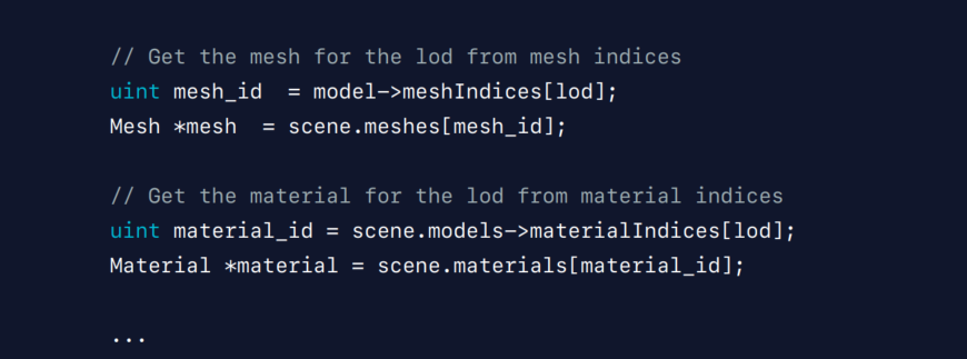
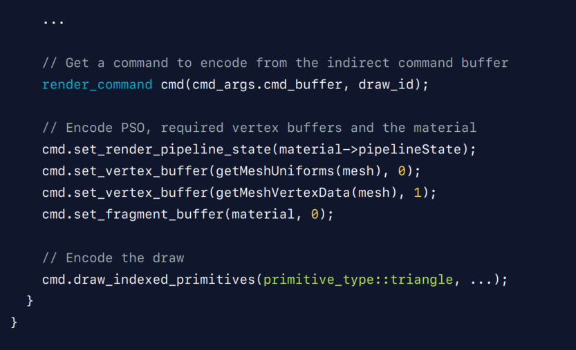
And we have acquired all the information we need; now it's time to encode.
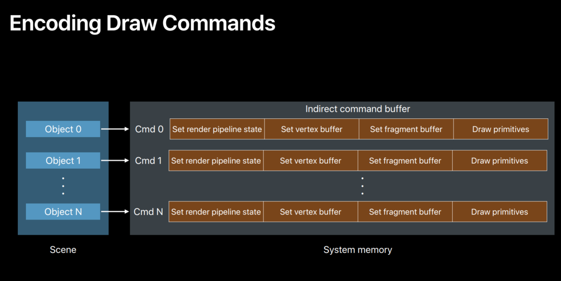
Let's just see what encoding into an indirect argument buffer, indirect command buffer really means.
So, indirect command buffer is an area of render commands.
Each command can have different properties.
A command can include a pipeline straight object that describes a shared pipeline and any vortex and fragment buffers that the draw call needs.
And the draw call itself.
So, encoding basically means that once we determine that an object is visible, we read it with all its properties and encode those into the indirect mine buffer.
Now, each thread that processes an object can encode into a particular slot in this indirect command buffer.
And since all threads are running in parallel, commands can be encoded concurrently.
Now, let's continue with our culling kernel example to see an actual example of the encoding.
Now, we first need a position in the command buffer to encode the raw command.
So, we use that raw ID to get ourselves a slot in the indirect command buffer.
And like we discussed, we need to set any parameters that the draw call needs.
Now, the material and mesh argument buffers that we just acquired have all the information we need to set the parameters.
So for example for material we can set the pipeline straight object that we need to set.
And from the mesh object, we can set any vortex buffer or any vortex uniforms that we need to set.
And of course the fragment needs the material, so we set that.
And finally this is how we encode the draw.
So that's it.
Encoding the draw call is very simple and easy.
Now, let's see how you can set up your path in your game.
Now, we first need an indirect command buffer to encode occluder draw commands, because that is the first thing that we talked about when we discussed our GPU-driven render loop.
So to render the occluders, we start up a compute dispatch that does custom culling of occulders and encodes the occluder draw commands.
And because each thread is doing independently encoding a draw, there can be multiple state settings, written and state settings in the indirect command buffer.
So, optionally we optimize the indirect command buffer to remove any driven end stage settings.
Now, this is a random pass that executes the occluder draws in the indirect command buffer.
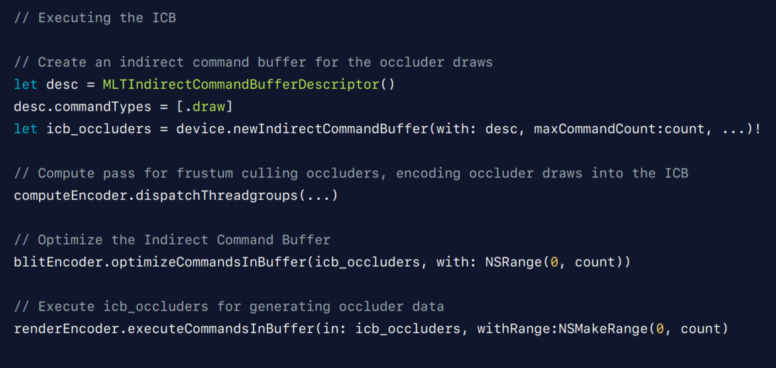
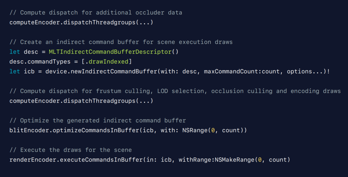
And similarly, the rest of the paths can be set up easily.
For example, here is our, the main compute dispatch that launches our culling kernel that we just talked about that does culling tests, LOD selection, and encoding draw commands.
Now we are ready to launch our final render pass that executes the commands in the indirect command buffer.
So that's it.
That's all it takes to draw the scene.
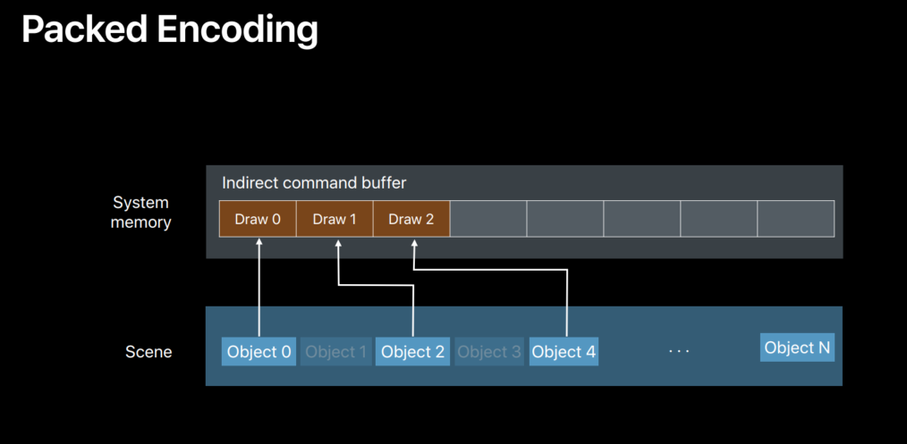
Now, let's take a look and see how the indirect command buffer looks like after the encoding of draw commands.
Now, it can be sparse with holes.
This is mainly because as we have just seen in our culling kernel example, the thread that is processing an object doesn't encode the draw command if it finds that object is not visible.
For example, objects one and three, in this case.
That means those slots in the indirect command buffer are empty.
So if you submit this command buffer to the GPU, it'll end up executing a bunch of empty commands, which is not really efficient.
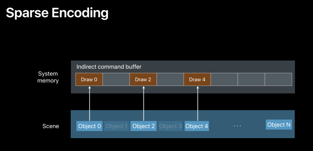
So, the ideal thing to do is to tightly pack the commands like this.
That is, we need a way to pack the commands as we encode the draws.
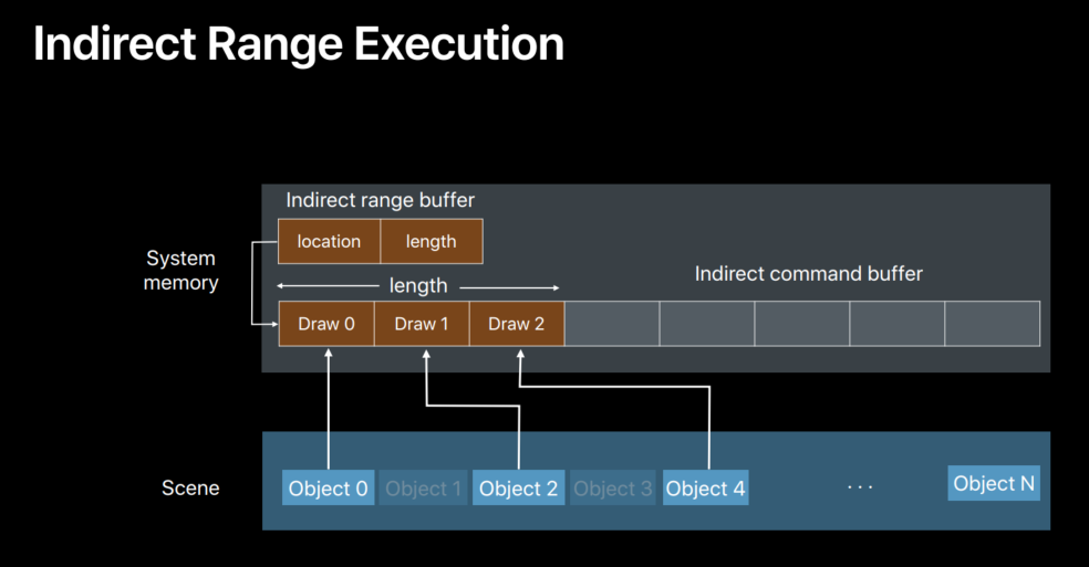
For that, we have indirect principle.
With indirect ranges, you can tell the GPU with execute call where to get the range of commands to execute.
Basically, you can have indirect range buffer that has a start location and number of commands to execute, and this buffer can be populated on the GPU as you're doing your encoding of draw commands.
And the execute call will pick up the start location and the number of commands from this buffer.
It can be used for both packing and the range.
Now, let's go to an example and see how this really works.
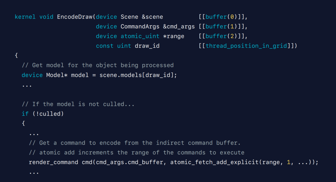
This is our culling kernel that we just discussed before, modified to use indirect range buffer.
Let's see how this kernel packs the draw commands.
We first pass in our pointer to the length member of the indirect range buffer.
And when we are retrieving the command to encode, we can automatically increment the length.
Now, each thread is atomically incrementing the length, and so when this compute work is done, the length is automatically set up in the indirect range buffer.
At the same time, the draw commands have been packed.
Because the indirect that is returned by this atomic instruction in this code is the previous value of the length.
And so for example, if you start at zero, the thread that is using the zero slot is incrementing the length to 1.
And the thread that is using the first slot is incrementing the length to 2 and so on.
So, this is great because now we not only pack the commands; we also updated the range at the same time.
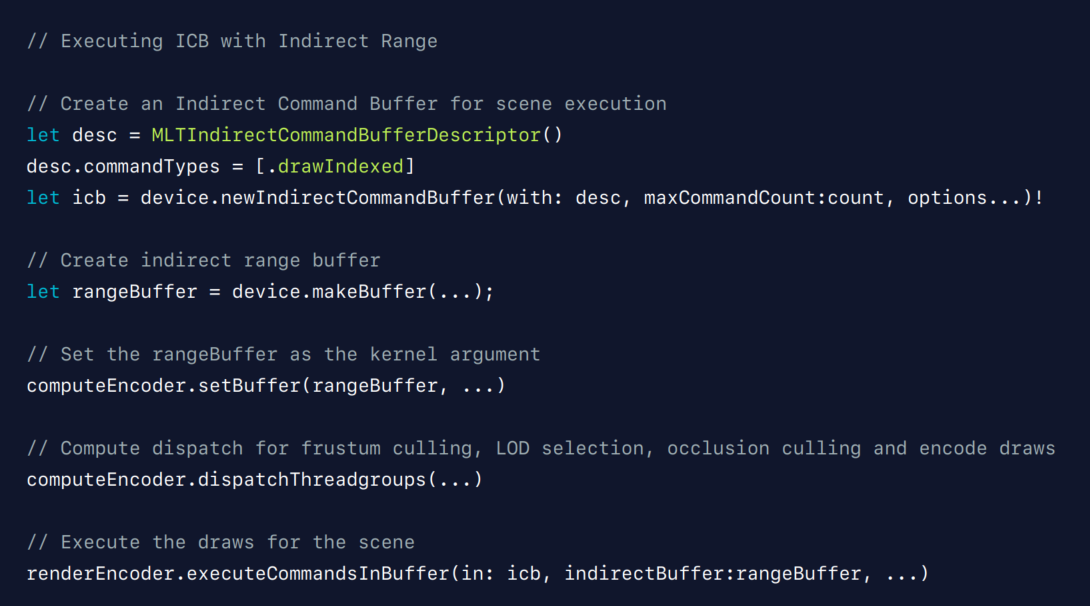
Now, let's see how we can set up the indirect range buffer in the application.
First, you create a range buffer for the compute pass to update the range.
Next, you set up the range buffer as a kernel argument for the culling compute kernel.
And then we do the compute pass that launches the culling kernel that does the object first thing and also updates the range automatically.
And finally, you schedule the pass with execute commands in buffer with indirect range API.
Now, this call will pick up the start location and the number of commands that is executed from this indirect range buffer.
So, with indirect ranges, you can get more efficient execution of indirect command buffers.
Now, so far in our GPU-driven pipeline, all these draw commands are built in compute passes on the GPU.
And these compute passes where regular dispatch is happening in your game.
So, one question that comes to mind is building compute dispatches on the GPU.
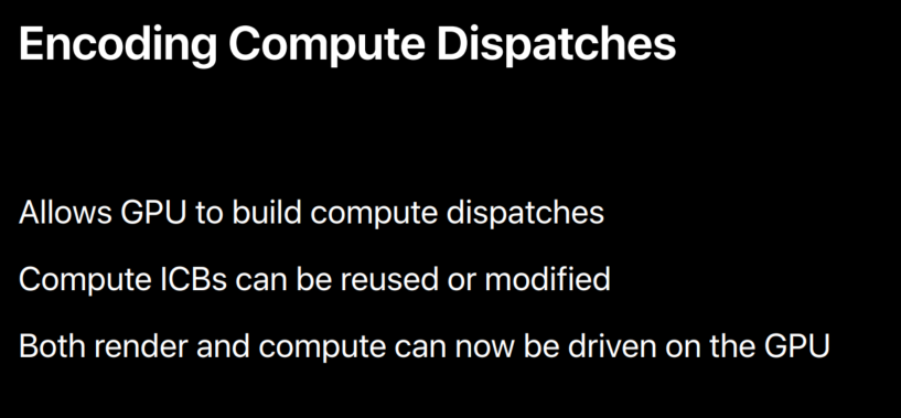
Can we encode compute dispatches into indirect command buffer? So, I'm very happy to let you all know that a new addition we are now putting into Metal 3 is support for encoding compute dispatches.
Now, you can build your compute dispatches on the GPU too.
In terms of functionality, compute indirect command buffers are just like render.
They can also be built once and can be reused again and again.
So, they also help in saving CPU cycles.
And the great thing is both render and compute can now be driven on the GPU.
It's really great because now you can build more flexible GPU-driven pipelines.
Now, let's see an example with this with the use case.
Per patch tessellation factors.
So, let's say we have a mesh that is made up of a bunch of patches and we want to generate tessellation patches for each patch.
We can definitely do this in the culling compute kernel that we talked about that does culling tasks and encodes draw commands.
That is a GPU thread that is processing an object can go through each patch of the object and can generate tessellation factors.
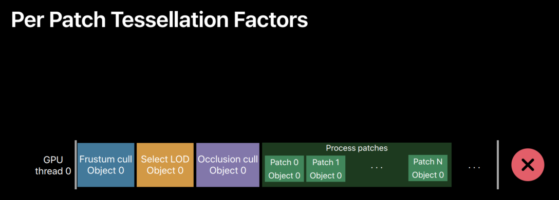
But that's not really an efficient thing to do because generating tessellation factors is also a paralyzable operation by itself.
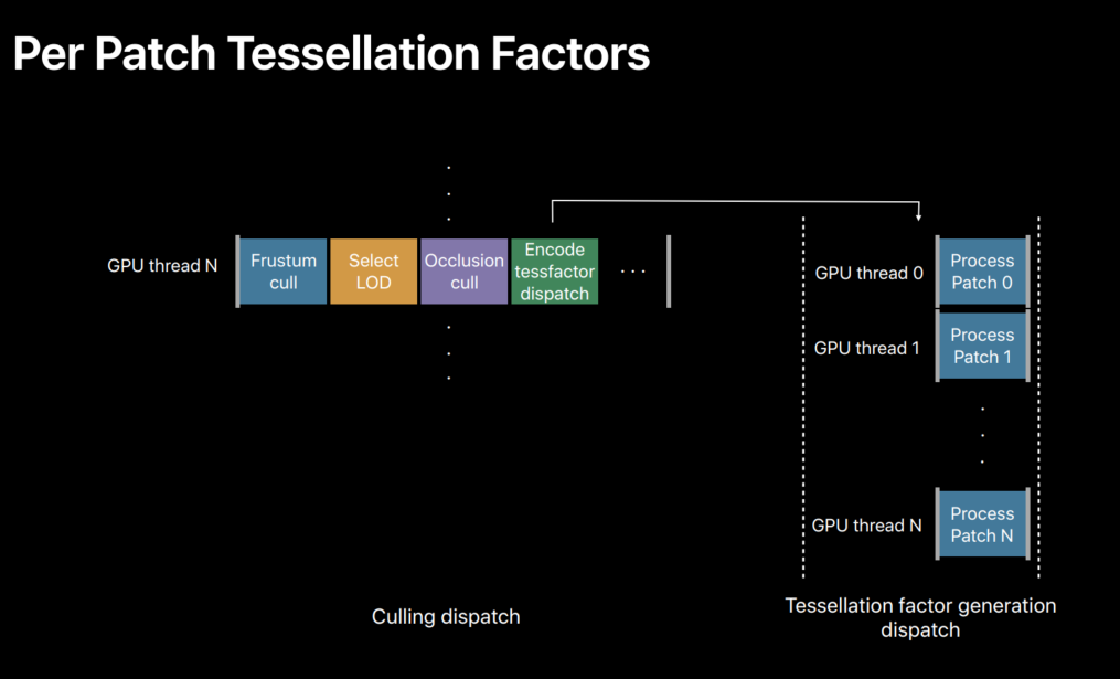
So, the efficient thing would be to distribute this per operation across multiple threads so that all patches are processed in parallel.
That is, each thread of the culling compute dispatch that is processing an object can encode compute dispatches for test factor generation.
And those dispatches can be executed on another compute pass, paralyzing the operation.
So, with GPU-driven dispatches, we can now do this.
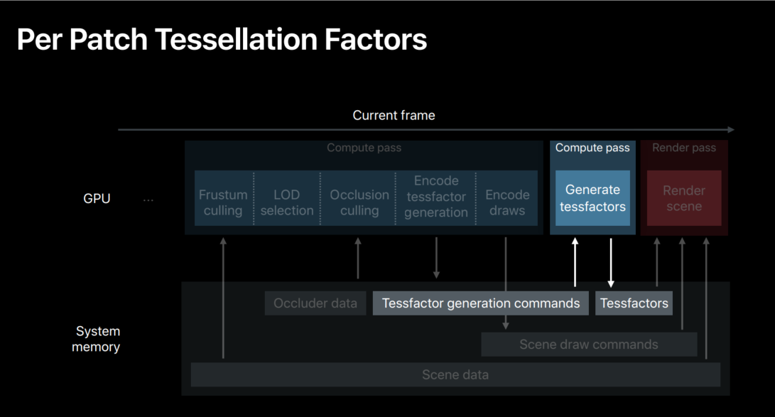
So, let's see how we can exchange our GPU-driven pipeline to accommodate this processing.
Here is the main compute pass that we talked about before that does the culling tasks, LOD selection and encoding of draw commands.

We can now action this pass to also encode dispatches for test factor generation.
For example, after a thread determines an object is visible, it can encode dispatches for test factor generation into an indirect command buffer.
And then those commands can be executed in another compute pass before the main render pass.
So, the GPU-driven dispatches combined with GPU-driven draws lets us build more flexible GPU-driven pipelines.
So, we built a sample to show you what we talked about in action.
Let's take a look.
Now, here is a bistro scene that you saw before.
This, we are actually doing a fly by through the street here.
This scene is made up of about 2.8 million polygons and close to 8000 draw calls.
And that's for one view.
And if you consider the shadow cascades that have been used here for shadow processing, this render is handling about four such views.
So, that is quite a few API calls if this scene gets rendered on the CPU.
But in this sample, we are using indirect command buffers and so everything is on the GPU.
It's completely GPU driven.
The entire render loop is on the GPU, and so it's saving the CPU from a lot of work.
Let's look at one more view.
Now, we are looking at the same view, same fly by, but we are looking at the camera as it's passing through the street here.
To be clear, we also are showing the camera that white object, that is the camera.
We are showing the geometry that is tinted with magenta color is, falling, geometry that is also the view for some of the camera.
So, as you can see, as the camera is passing through the street, there's quite a bit of geometry that is also the view frustum of the camera.
And our culling compute dispatch that does frustum culling on the GPU determined this geometry, this tinted geometry as invisible.
And so this geometry doesn't get processed or rendered on the GPU, saving significant rendering cost.
Let's look at one more final view.
And here is one more view.
Here we are showing both frustum and occlusion culling at work.
We are, we tinted the geometry that is occluded with cyan color and the geometry in magenta is outside the view frustum.
And you can see there's quite a bit of geometry on the right here that is occluded by the bistro, so it is in cyan color.
And as you can see, there's a lot of geometry here.
Also the view frustum are, is occluded.
And again, our culling compute kernel that does both frustum and occlusion culling on the GPU determined these geometry to be invisible.
So, this tinted geometry doesn't get processed or rendered on the GPU, saving significant rendering cost and increasing performance.
Simpler GPU Families
So, before we end this talk, I'm going to show you one more thing.
I'm going to show you how we are making it easier than ever to write a cross ref on Metal core.
I'm also going to show you how to more easily target features that are iOS, tvOS and macOS specific.
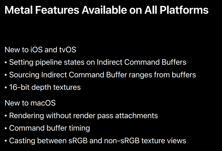
And before we do that, let's take a quick look at Metal features that are now available across all our platforms.
Now, we have several features new to iOS and tvOS.
In the previous sections, we showed you how setting pipeline states in indirect command buffers helps you to fully utilize GPU-driven pipelines.
We also showed you how indirect ranges allow you to more easily and more efficiently pack and execute indirect commands.
And finally, we are bringing 16-bit depth texture support to iOS and tvOS.
This has been a popular request that helps to optimize shadow map rendering.
We also have several important features new to macOS.
We can render now without attachments in cases where you need more flexible outputs to memory buffers.
You can query the time your command buffer takes on the GPU so you can adjust your representation intervals dynamically.
And finally, macOS now supports casting between sRGB and non-sRGB views to better accommodate linear versus nonlinear lighting.
So, now let's take a look at the new GPU family API.
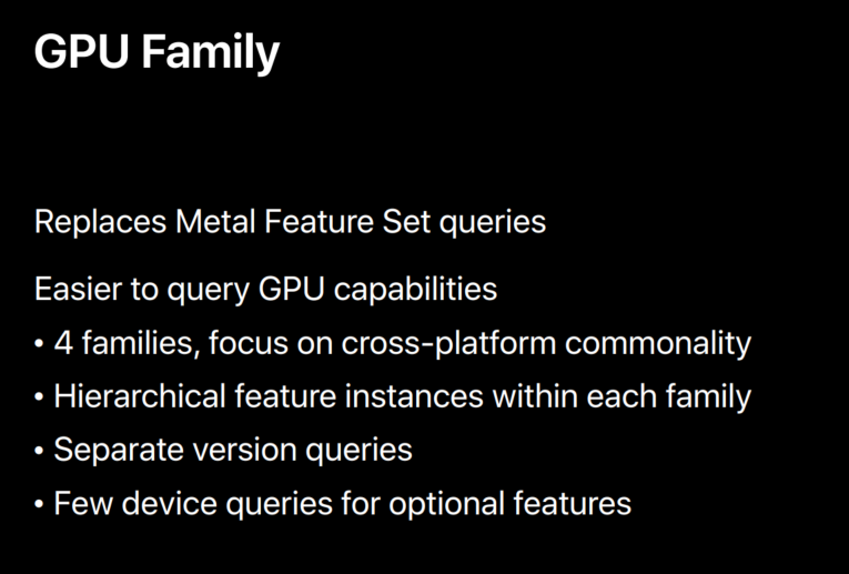
Now, you previously used Metal feature set queries to condition your applications based on available features and limits.
But the number of features, feature sets has grown and they currently number, numbers in the dozens.
The GPU family queries replace feature sets and makes it easier to query the capabilities of the system.
First, we have consolidated into four families and organized them to simplify cross-platform development.
Second, each family supports a hierarchy of features organized into one or more instances.
So, support for one instance means all earlier instances are supported.
Third, the new API separates out Metal software version query to track how to instances of a given family change our software delivers.
And finally, a GPU family defines a small set of device queries for optional features that don't neatly fit into families.
Now, with that said, let's take a closer look at the new GPU family definitions.
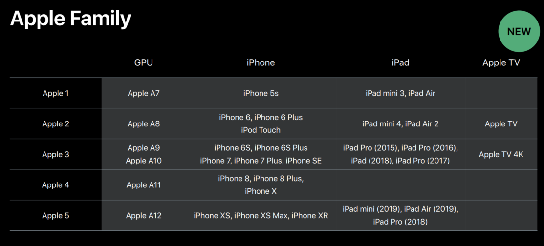
All iOS and tvOS features are now organized into their family, a single family of five instances.
With each instance supporting all features included within the earlier instances.
So, I'm not going to enumerate all the features here, but the resource section of this talk will have a table that'll map features to families and instances.
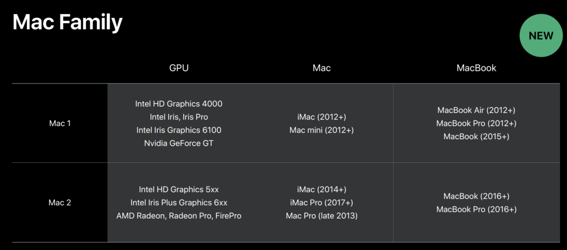
Mac features are similarly organized around only two instances.
Again, the Mac II supports all the features from Mac I.
Now querying these features, these families greatly simplifies writing flat, unspecific code.
But what about when you want to target all of the platforms? For that, we have the new common families.
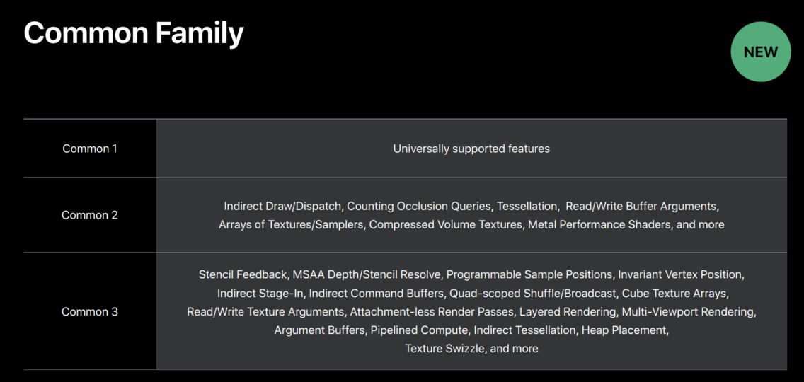
The common family organizes Metal features into cross-platform hierarchy.
Common 1 is universally supported by all Metal GPUs and is a great choice for apps that only use Metal lightly.
Common 2 provides all the building blocks necessary for great game development such as indirect draw, counting occlusion queries, tessellation, and Metal performance shadow support.
And common 3 provides all the features needed by advanced applications such as indirect command buffers, layered rendering, cube map arrays, and vortex position invariants.
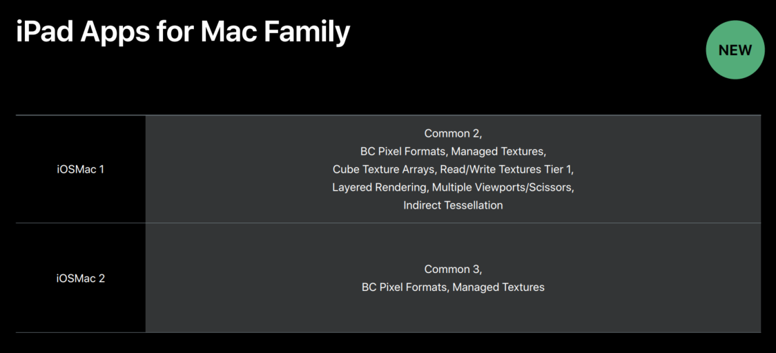
And finally, Metal 3 provides a special family for iPad apps targeting the Mac.
That is, tuned for that experience.
The two iOS mac instances support a combination of features critical for great performance on the Mac.
In particular, they make available the Mac-specific block compression pixel formats and manage texture modes for use within an otherwise completely iOS application.
Now, iOS Mac 1 supports all the features of Common 2 plus several features from Common 3.
Besides the BC pixel format and managed textures, it supports cube texture arrays, read/write textures, layered rendering, multiple viewport rendering, and indirect tessellation.
iOS Mac II supports all the features of Common 3 in addition to the BC pixel formats and managed textures.
So, that's the four new families.
Now, let's take a look at how you'll use the new QD API in practice.
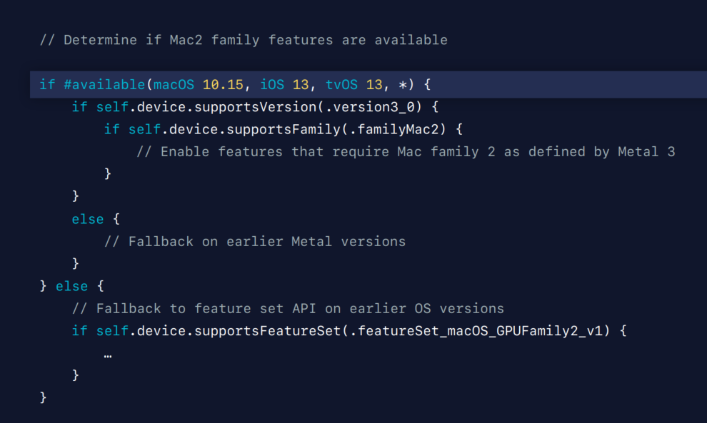
Now, in this example we'll check whether the Mac II features are available.
We start by checking whether the OS supports the new family API.
And if the new family API is available, then we use to check for Metal 3 features that are available.
Since Metal 3 is new, you don't need to strictly check for it, but that's a good practice.
And if Metal 3 is available, then we check for the family we would like to use.
Cross-platform applications here, check for one of the common families, as well as one or more Apple or Mac-specific families.
If either the API or the version are not available, then we fall back to the older feature set API on earlier Metal versions.
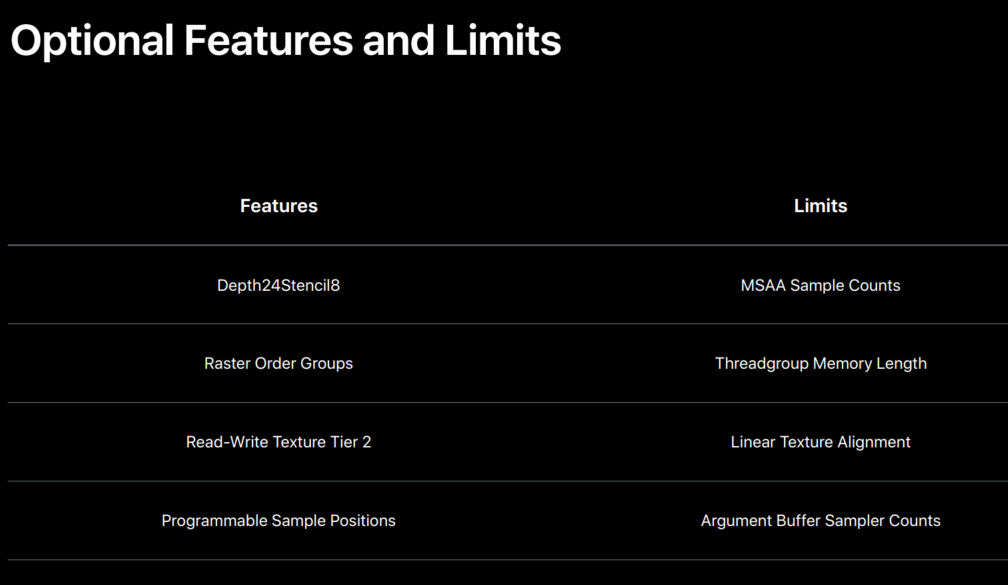
So, now let's take a look at the setup option features you can query for.
Now, when a family specifies a general behavior of GPUs in that family but some important features and limits are not supported uniformly across a family.
Such as a depth 24 stencil 8 pixel formats, and the number of MSA samples in a pixel.
So to handle those cases, the Metal device provides an API to query for each of those features directly.
But as you can see, that is not many features that fall into this category.
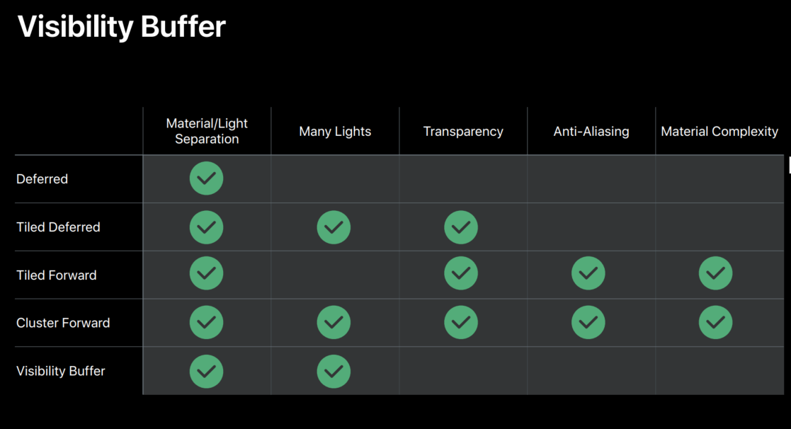
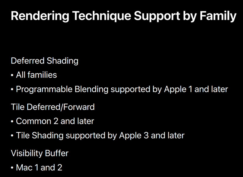
So, to end this section, let's look at how the many techniques we have discussed so far are supported by the new GPU families.
Classic deferred shading is supported across all our platforms and programmable blending is supported across all Apple GPUs, making it a good default choice for your games.
Tile deferred and forward rendering are also broadly supported with Apple-specific optimizations requiring more recent hardware.
And finally, the visibility buffer technique is only supported by the Mac family.
It just happened to have very demanding resolution requirements.
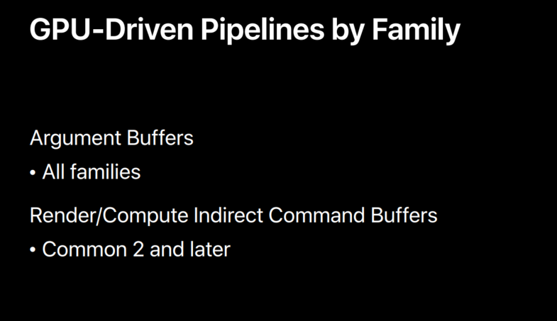
Now, let's end this section by looking at how our GPU-drive pipeline features are supported across our families.
Now, some features require broad support to become a core part of render engines, and we believe that GPU-driven pipelines require that kind of support.
So, we are therefore very happy to let you all know that argument buffers and indirect command buffers for both graphics and compute are now supported by a Common family 2 and later.
Now that brings us to the end of this session on Model Rendering with Metal.
We hope you can apply all these techniques to your games and apps.
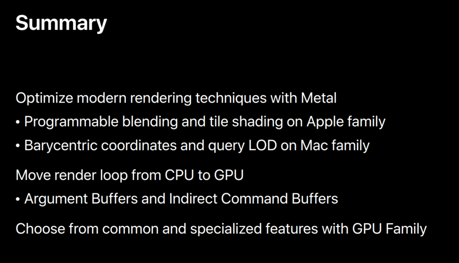
Let's do quick recap.
My colleague, Jaap, just showed you how to implement many advanced rendering techniques with Metal, techniques like deferred shading, tile forward rendering are excellent matches for iOS when combined with and optimized with programmable blending and tile sharing.
On Mac, you can use the new barycentric coordinates and query LOD to implement the visibility buffer technique and render it high resolutions.
But no matter what technique you choose to use, you can move your entire render loop to the GPU.
Frustrum culling, occlusion culling, LOD selection, can all be done on the GPU with argument buffers and indirect command buffers.
And now we can also encode compute dispatches into indirect command buffers on the GPU.
Whether you want to target a wide range of hardware on both iOS or macOS, or only want to use a few advanced Metal features, you can now use the newly redesigned GPU family API to check for feature availability at runtime.
Now, please visit our session website to learn more about Metal features and GPU-driven pipelines.
We will be posting the sample app that we used in this talk.
You can explore those techniques and integrate them into your apps and games and please join us in our labs.

In fact, there is one right after this talk.
Thank you, and have a great conference.
虽然并非全部原创,但还是希望转载请注明出处:电子设备中的画家|王烁 于 2022 年 5 月 25 日发表,原文链接(http://geekfaner.com/shineengine/WWDC2019_ModernRenderingwithMetal.html)