本节内容,来自Metal Enhancements for A13 Bionic
关联阅读:
Jaap van Muijden: Welcome to Metal Enhancements for A13 Bionic.
My name is Jaap van Muijden, from the GPU Software team at Apple.

Today I’m going to introduce you to the latest Apple-designed GPU in the A13 Bionic, and the new Metal features it enables.
I will then then show you how to use those features to reduce your app’s memory usage, and optimize its run-time performance.

The new A13 Bionic continues the rapid evolution of Apple-designed GPUs by focusing on three major areas: general performance, architectural improvements that better meet the evolving needs of modern apps, and advanced Metal features.

Let’s take a look at each.
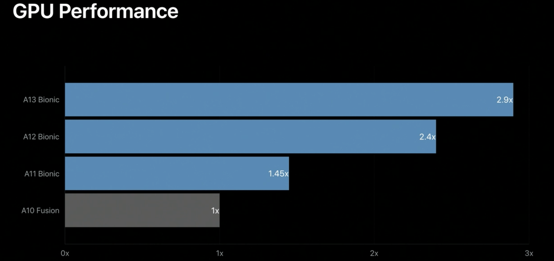
The GPU in A13 Bionic is almost three times faster than the A10 Fusion in general performance, and builds on the great performance improvements of the A11 and A12 Bionic GPUs.
Existing apps run faster on the A13 and can complete each frame in less time, which in turn leads to power savings and extended app usage.
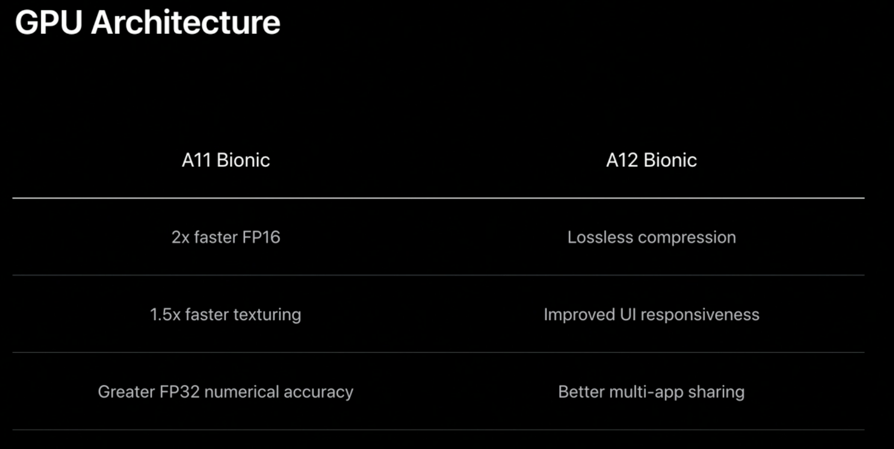
The Apple-designed GPU architecture has quickly evolved to better meet the demands of modern apps.
Beginning with the A11, the 16-bit floating point and texturing rates were increased to alleviate common bottlenecks in games, and the numerical accuracy of 32-bit floating point operations were improved to better handle advanced compute workloads.
The A12 GPU greatly improves memory bandwidth by losslessly compressing and decompressing texture content to and from memory.
It also adds dedicated hardware to support the user interface, ensuring even faster response times, but also reducing the impact of UI elements on foreground apps.
And the A12 and later GPUs enhance the iPad experience by sharing its resources between apps more efficiently.
And now we have the A13 GPU.
The A13 GPU architecture greatly improves the processing of high dynamic range content on the GPU, by doubling the rate of 16-bit floating point operations and adding support for small 16-bit numbers that better preserve black levels.
The A13 GPU also provides significantly better support for independent compute work that executes concurrently with rendering workloads.
Apple-designed GPUs have supported this asynchronous compute capability since the A9, but the A13 GPU takes it to the next level by adding more hardware channels and minimizing impact to the more deadline-sensitive rendering tasks.
Now before we describe the new Metal features of the A13, let’s also quickly recap some of the major Metal features introduced on the A11 and A12 GPUs.

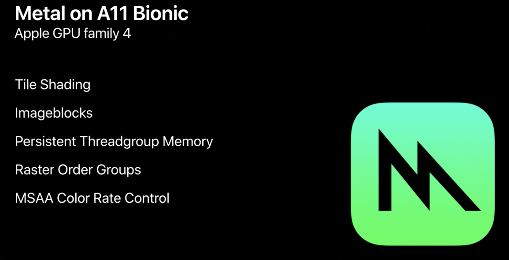
Let’s start with the A11.
Tile shading, imageblocks, and persistent threadgroup memory all are features designed to explicitly leverage Apple’s tile-based deferred rendering architecture and work together to optimize the bandwidth usage of many modern rendering techniques.
Rasterization order groups allow you to manage complex, per-pixel data structures on the GPU, and color rate control optimizes the use of multi-sample anti-aliasing in advanced rendering algorithms.
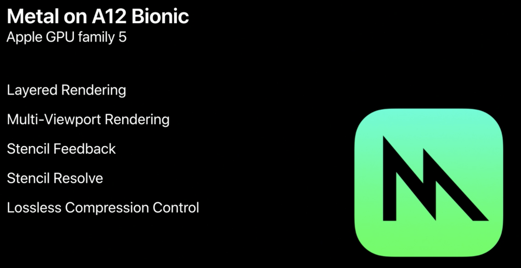
And now on to the A12.
Layered rendering lets each rendered primitive target a unique slice of a 2D texture array, while multi-viewport rendering lets each primitive do the same for up to 16 viewports and scissor rectangles.
Stencil feedback lets each fragment set a unique stencil reference value for advanced per-pixel effects, while stencil resolve allows for stencil buffer reuse across MSAA and non-MSAA passes.
And although lossless compression is enabled by default wherever possible, Metal also provides direct control over in-place compression and decompression of shared storage mode textures when optimal readback is required.
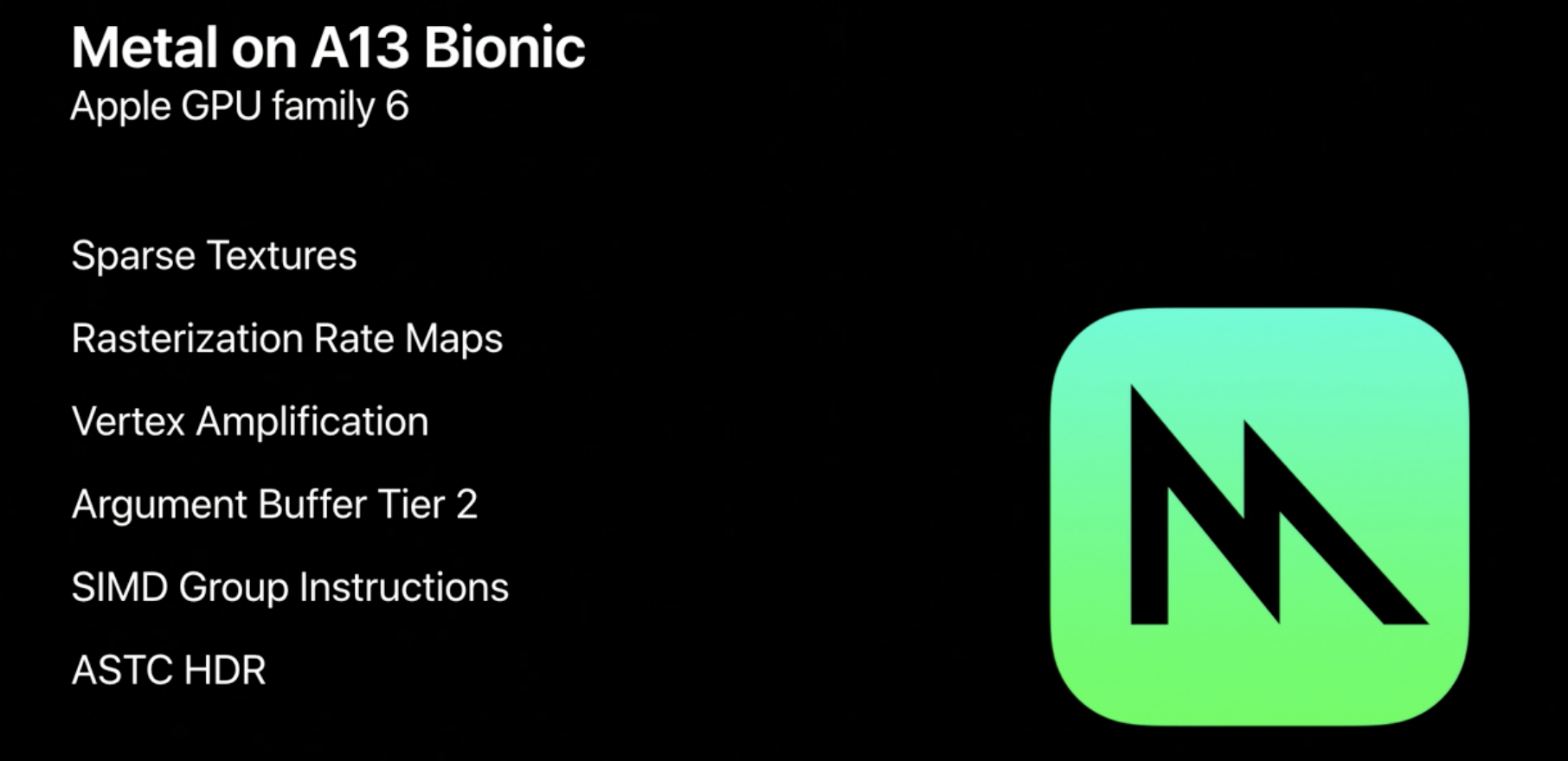
So now let’s introduce the new Apple GPU Family 6 that supports the A13 GPU.
Sparse textures enable higher-quality texture streaming for open-world games at a fixed memory budget, by tracking the most important regions of each texture and then mapping only those regions to memory.
Rasterization rate maps focus high-quality rasterization and shading to the image areas that matter most, while reducing rates elsewhere, saving both memory and performance.
Vertex amplification eliminates redundant vertex processing that would otherwise occur with layered renders that share geometry.
GPU-driven pipelines enable you to draw larger and more immersive scenes, and with argument buffer tier 2, apps can execute their GPU-driven workloads more flexibly than ever before.
SIMD group instructions optimize sharing and synchronization among the threads of an SIMD group during shading.
And ASTC HDR brings high-quality lossy compression to high-dynamic range textures, saving significant memory and bandwidth.
sparse textures
Let’s look at each of these in more detail, starting with sparse textures.
Sparse textures is a brand new feature introduced on the A13 GPU that let you control the storage and residency of Metal textures at a fine granularity.

Sparse textures are not fully resident in memory.
But instead, you can allocate sections of them on a special memory heap called a sparse heap.
Here you can see two sparse textures that have parts of their data allocated in such a sparse heap.
A single heap can provide storage for many sparse textures, all sharing a single pre-allocated pool of memory.
All sparse textures are split up in units called sparse tiles, which have the same memory footprint independent of texture resolution or pixel format.

So what are the applications of this feature? One of them is texture streaming.
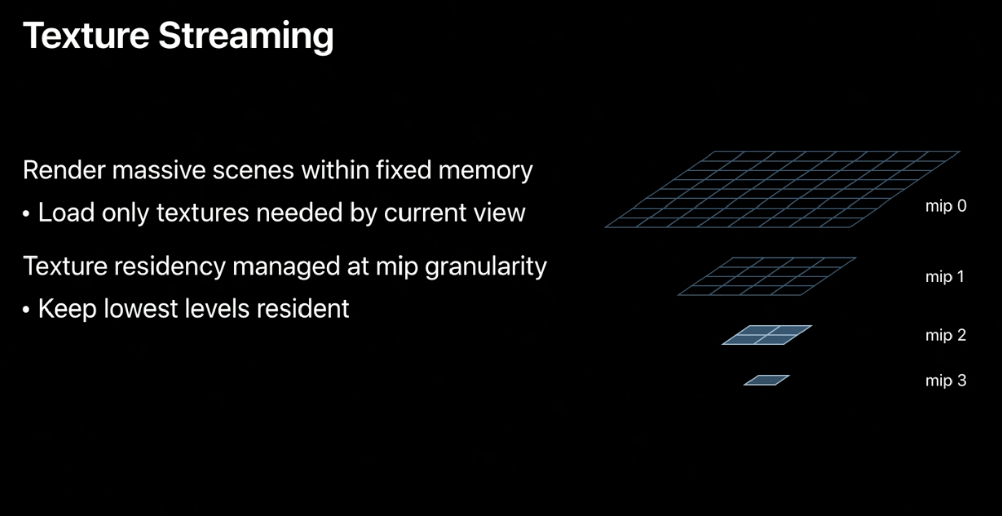
Texture streaming lets you render incredibly large scenes with a fixed memory footprint by loading only the texture mipmaps that are needed for the current view.
With traditional texture streaming, individual mipmaps are loaded when required and evicted when no longer needed, or when more important textures need the memory.
Texture streaming traditionally manages texture residency at mipmap granularity.
The lowest levels of the mipmap pyramid are kept resident in case a higher quality mipmap is requested, but not yet streamed in.
It may not be available yet because the loading operation has not completed, or there is insufficient allocated streaming memory.
Having the lowest level mipmaps available ensures that there is always some valid data to sample, even though it is of lower resolution.
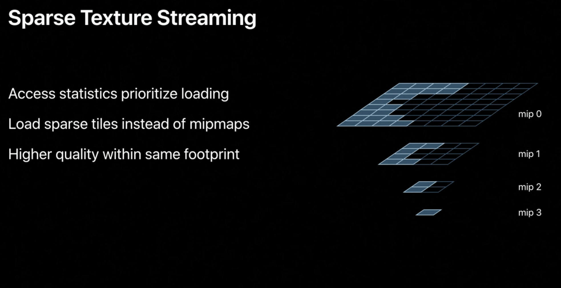
Metal’s sparse texture feature improves on this texture streaming model in two ways.
First, sparse textures provide texture access counters that you can use to determine how often each region of a sparse texture is accessed.
This lets you prioritize texture loading, as regions that are accessed more often by the renderer are generally more visible in the current view.
Secondly, residency can be managed at the sparse tile granularity instead of mipmap granularity.
This lets you be even more efficient with your texture memory, and allows for more visible texture detail where it counts.
Taken together, sparse textures let you stream more visible detail with the same memory budget, improving quality.
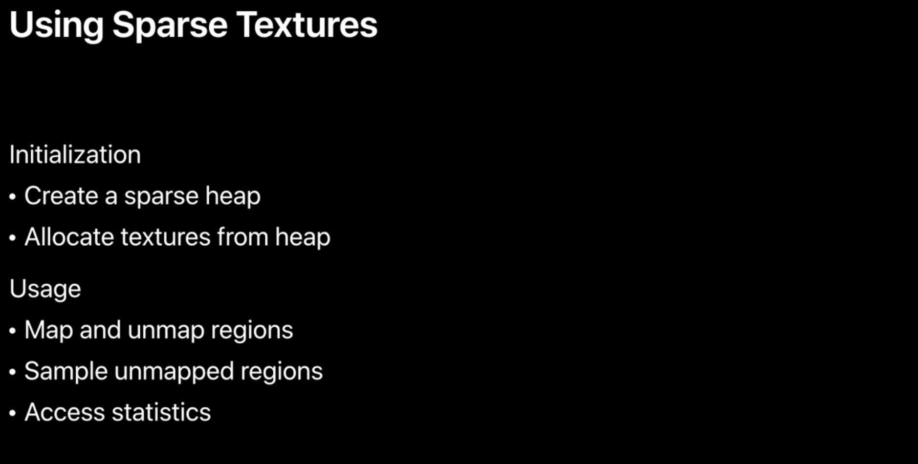
Now let’s look at how you create and use sparse textures in Metal.
To start using sparse textures, you first create a sparse heap and then allocate one or more textures from it.
New sparse textures are created initially without any mapped sparse tiles.
You need to request memory mappings from the heap using the GPU.
The memory is mapped in tile-sized units called sparse tiles, similar to virtual memory pages.
Likewise, you need request the GPU to unmap tiles when they are no longer needed.
Sampling a sparse texture works just like a regular texture, and sampling unmapped regions return zeros.
Finally, the texture access counters can be read back from a sparse texture, to get estimates for how often each tile is accessed, so that you can precisely control and prioritize when you map tiles for your textures.
Let’s look at each of these steps in more detail.
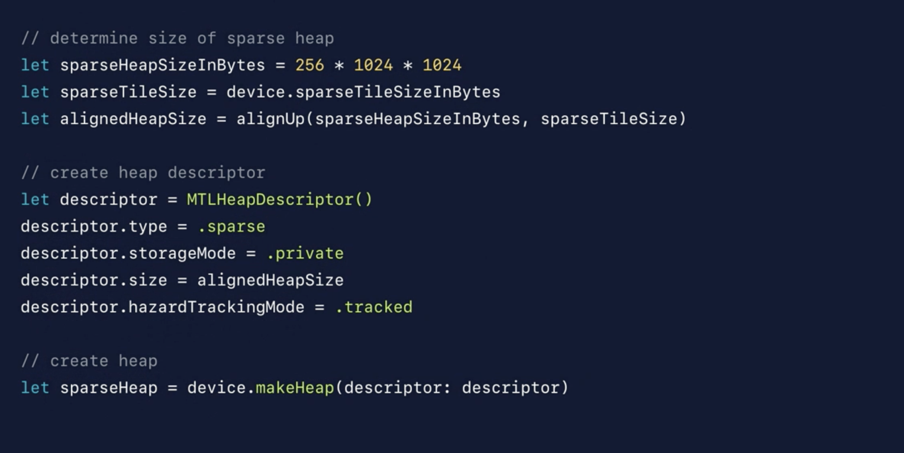
Here we have some Metal code that creates a sparse texture heap with a given memory size.
We first calculate the size of our heap, and make sure it is a multiple of the sparse tile size.
Here we use a local helper function to round up our data size to the nearest multiple of the sparse tile size.
We can then generate the sparse heap descriptor; we set the heap type to sparse, and specify the size of our heap in bytes.
We then create the sparse heap using our MTLDevice object.
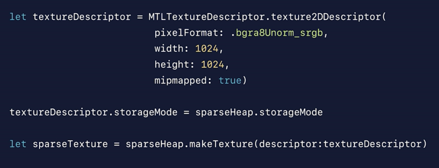
Creating a sparse texture is very easy.
First, we create a texture descriptor as normal, and then we create the texture using the sparse heap object.
Now that we have seen how you can create the sparse texture, let’s take a look at how to map regions onto memory.
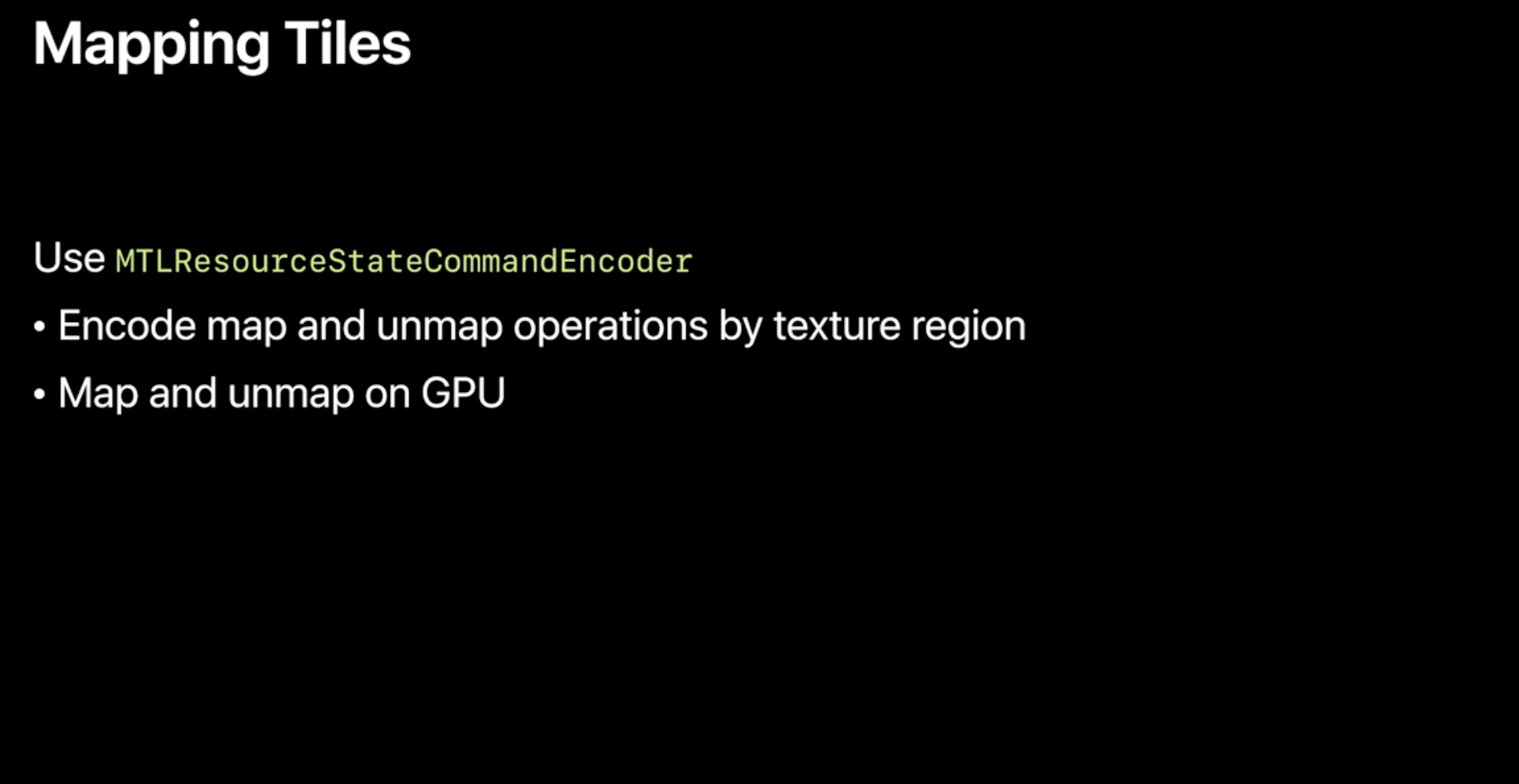
The mapping and unmapping of regions of a texture is done by encoding map and unmap commands in a resource state command encoder.
This encoder can be used to schedule the map and unmap operations on the GPU timeline, similar to encoding other render commands in Metal.
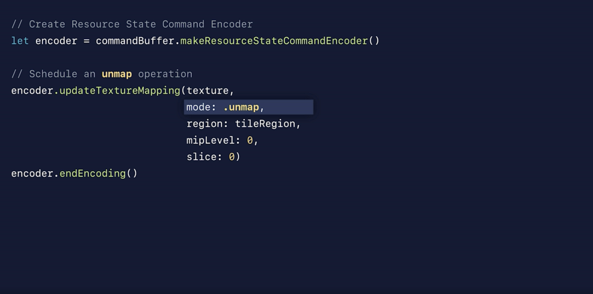
Let’s see how this looks in code.
First we create the encoder.
And then we simply encode a map operation; we specify the texture and what regions, slice, and mip level of the texture we want to map.
The region is now mapped, and you can blit or create your texture data onto the mapped memory.

To unmap a section, we follow the same procedure; the only difference is the mode of the update we encode.
Now that you have created and mapped our texture data, let’s move on to the sampling of sparse textures.
Sampling from a sparse texture is no different than sampling from a normal texture.
There is well-defined behavior in case an unmapped section is accessed.
Sampling an unmapped region returns a vector of zeroes, and any writes are discarded.
In addition to the standard sampling functions, Metal provides a sparse_sample function that can be used in shaders to test for unmapped regions.

Now that you’ve seen how to create, map, and sample sparse textures, let’s look at a simple implementation.
One way to efficiently sample sparse textures is to perform fallback sampling.
In your shader, you can first try to fetch texels using the sparse_sample method, and if that fails, you can fall back to a lower-level mipmap.
By always keeping the lower mipmap loaded, you are guaranteed to find a valid sample.
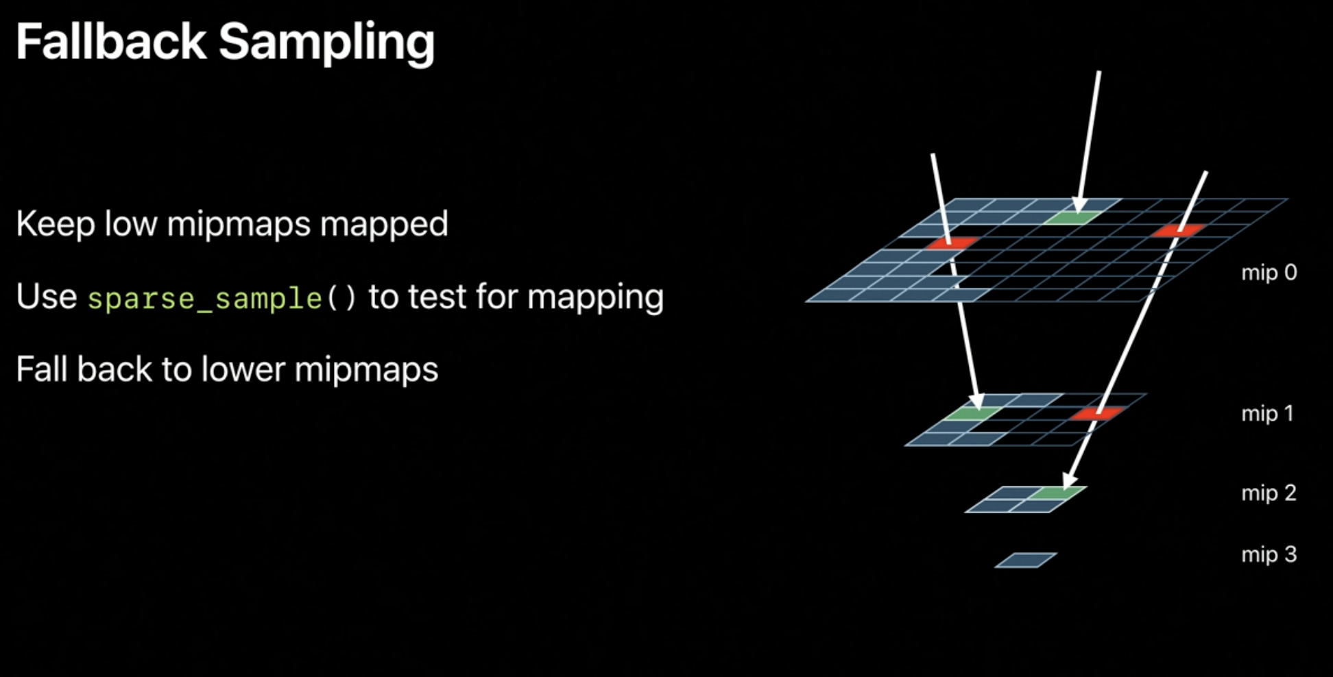
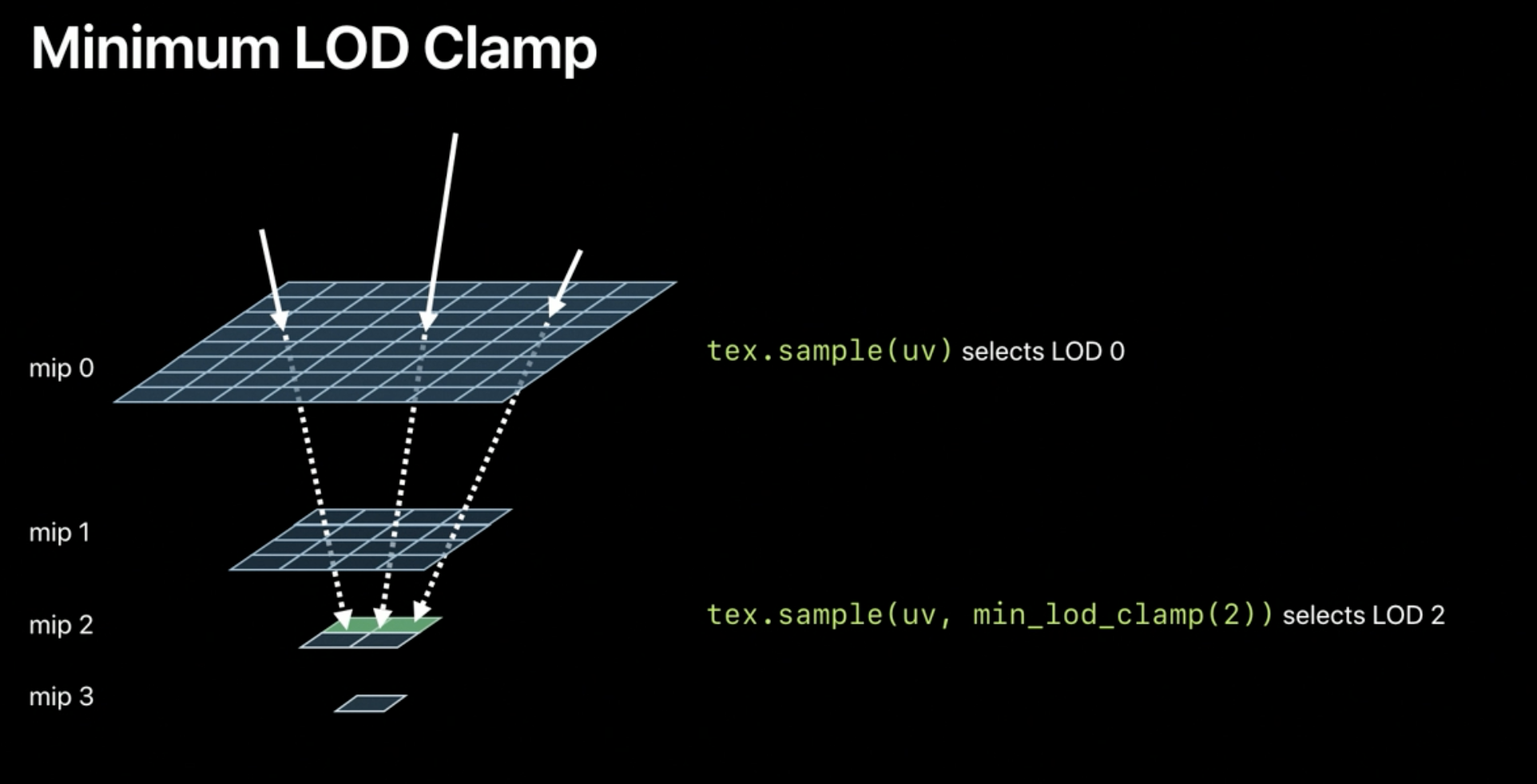
And to better support fallback sampling, the Metal shading language also supports a new argument on texture methods called min LOD clamp.
Min LOD clamp lets you set the highest mipmap in the chain that can be accessed.
This lets you guarantee a valid sample by specifying the highest mipmap that you know you have data for.
Let’s look at that in code.
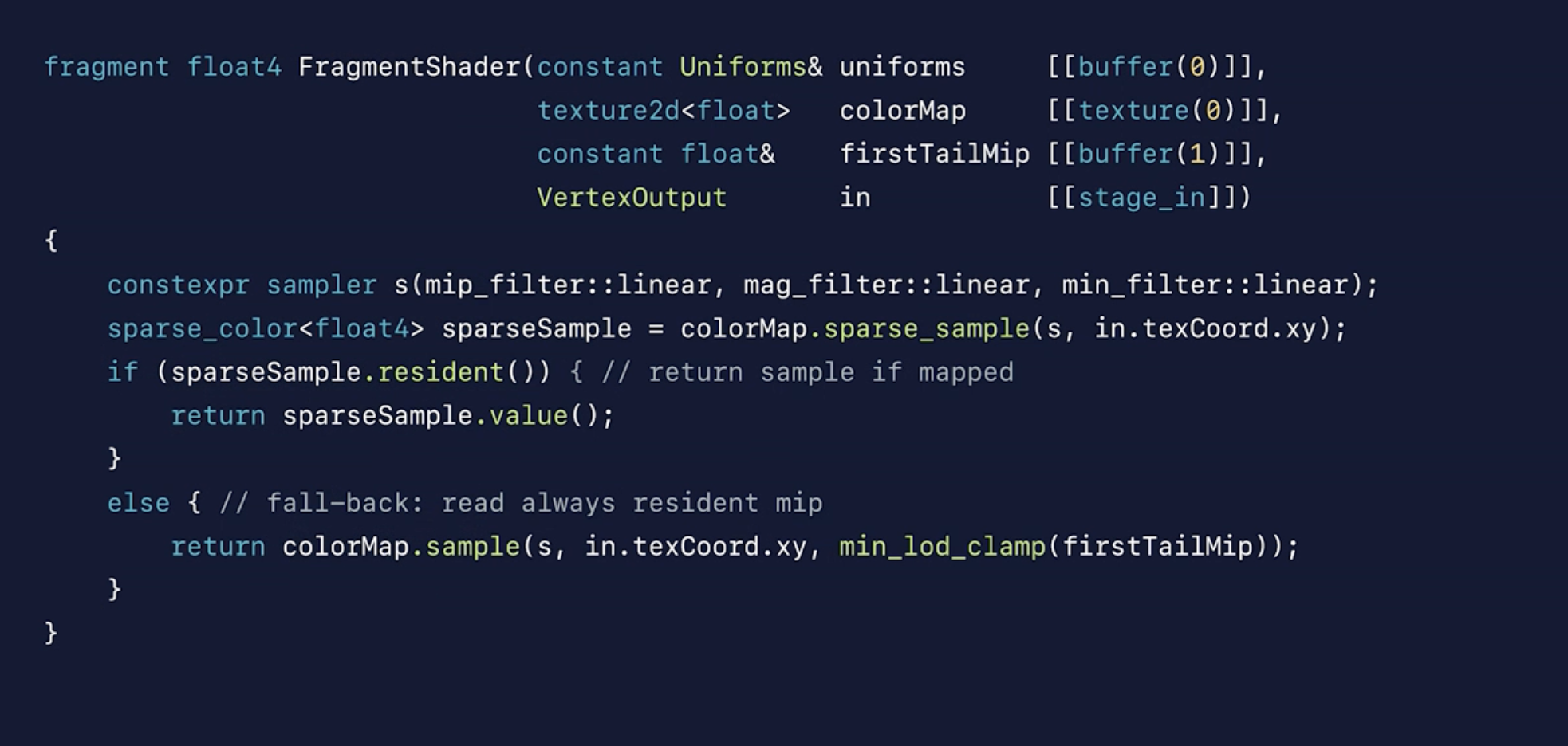
Here we have a fragment shader that samples from a sparse texture.
You start sampling your sparse texture using the sparse_sample method, which returns a sparse_color object.
You can then call the resident method on the returned object to determine if the GPU sampled mapped data.
If it did, you retrieve the sampled value and return it.
Otherwise you sample the sparse texture again, but this time with an LOD clamp to force the sampler to bypass higher mipmaps.
Since you guaranteed that this mipmap and lower mipmaps have data, the second sampling call is made using the normal sample method.
Now that you’ve seen the functions for mapping and sampling sparse texture data, let’s talk a little bit about how to decide when to map or free sparse texture tiles.
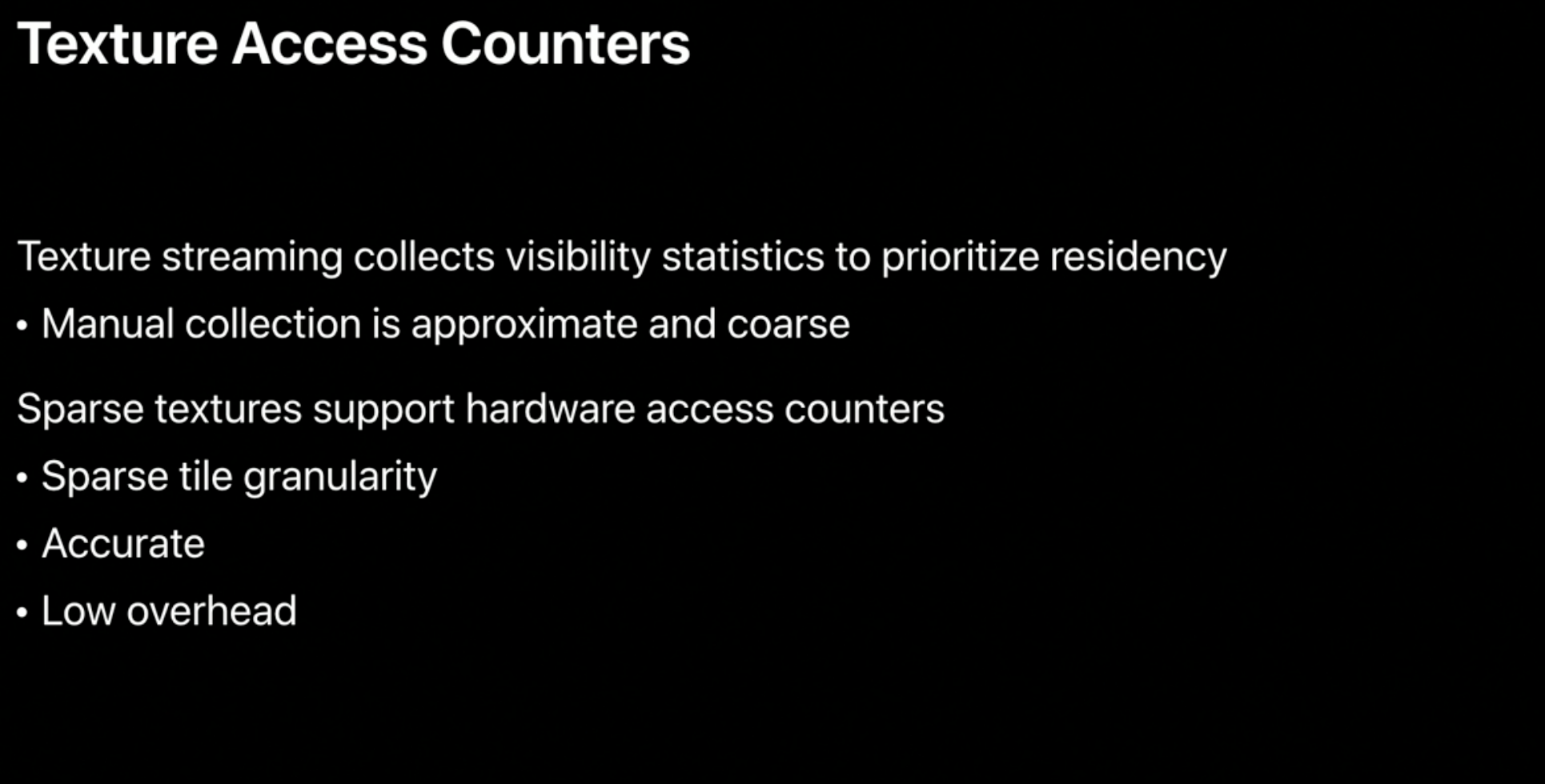
Traditional texture streaming systems manually collect app-level statistics to help prioritize texture residency.
These methods are often coarse at the mipmap or mesh granularity to help manage the overhead.
Metal instead supports a fine-grained solution called texture access counters.
These counters accurately track how often sparse tiles are accessed by the GPU with very low overhead.
Texture access counters are queried from the GPU.
Let’s look at how this works.
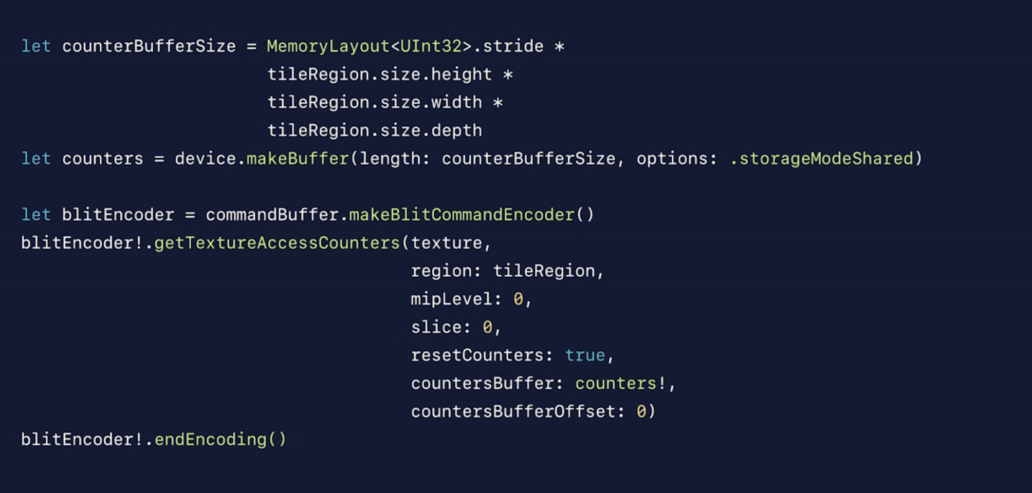
This Metal example will collect the texture access counters from the GPU.
You start by creating a buffer to contain the sampled counters.
And then you encode a blit to copy the counters from our sparse texture to our buffer, specifying the mip level, slice, and region you’re interested in.
Traditional texture streaming techniques have served us very well over the years, and given a fixed memory budget, we can stream in the mip levels for the textures that user sees.
When the texture budget gets exhausted, we can no longer stream in higher resolution mip levels and we start seeing uniformly blurry textures.

But with sparse textures, you can now get a better usage of your memory.
You can map the memory to make room for the individual texture tiles that the user sees, at the quality level that is most appropriate for each texture tile within a given mip level.
This allows you to distribute texture memory for the tiles that make the most visual impact.
Additionally, this feature saves bandwidth when streaming textures, as the sparse texture API allows you to map and unmap individual tiles instead of having to copy and rearrange entire mipmap chains in memory during streaming.
That’s it for sparse textures, a really important memory optimization that will also improve texture streaming quality.

rasterization rate maps
Now let’s move on to the runtime optimization technique called rasterization rate maps.

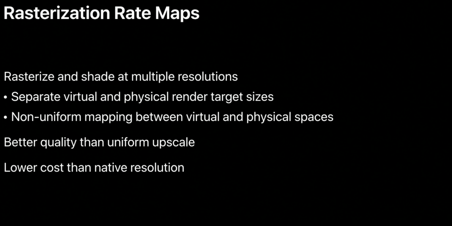
Rasterization rate maps let you make better use of Retina displays by rasterizing and shading the image areas that matter most at highest resolution, while reducing quality where it's not perceived.
Rasterization rate maps let you rasterize and shade at multiple resolutions by defining both a screen space and physical render target size, and a nonuniform mapping between the two spaces, to control the quality of each region.
The physical resolution is smaller than the screen space, saving bandwidth and reducing the memory footprint.
And the nonuniform mapping results in higher-quality visuals than the uniform upscale often used in games at a fraction of the cost of rendering the entire screen at native resolution.
Let’s take a closer look at how this works.
Here is a screenshot of a diffuse layer from the g-buffer of a sample renderer.
Traditional rendering draws geometry by calculating the screen space coordinates of each vertex, and then rasterizing the resulting primitives in screen space to produce fragments.
These screen space coordinates have a one-to-one mapping to the coordinates of the physical render target during rasterization.

With rasterization rate maps, you can configure the rasterizer to map screen space coordinates unevenly when creating fragments thus reducing the number of total fragments produced and simultaneously rendering to a smaller render target.
In both images, the white grid corresponds to an evenly spaced grid in virtual screen space.
But as you can see here, it is distributed unevenly in physical space.
In this example, we’ve used rasterization rate maps to keep the screen resolution in the center of the screen, but reducing it towards the edges of the screen.

To see this more clearly, let’s zoom in on one of the center tiles.
The resolution of this physical tile matches the resolution of the same region within the g-buffer.
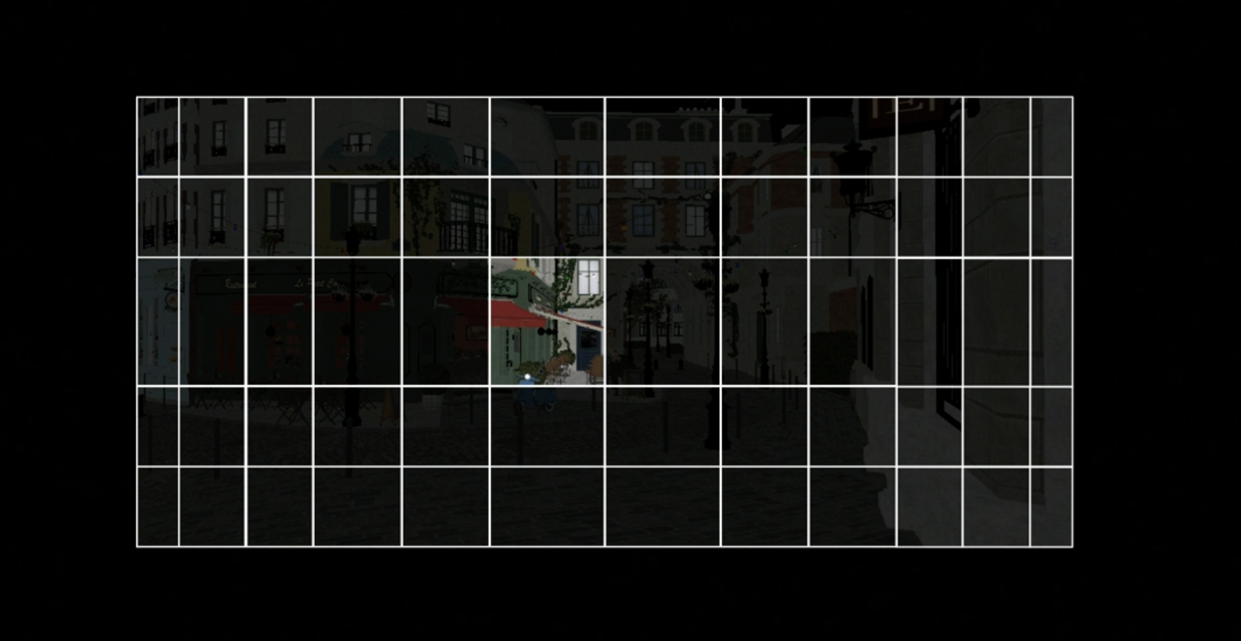
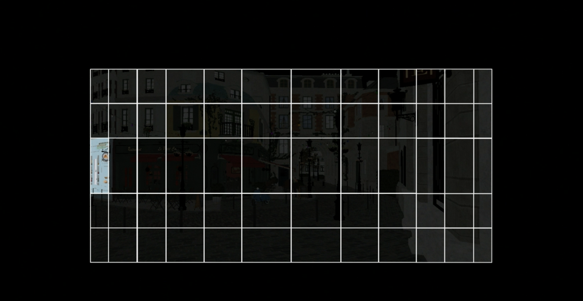
But as you move towards the edge of the screen, the quality is reduced by effectively reducing the physical space dedicated to that tile.
This leads to a distorted image in your physical image, but we will show that this mapping can be reversed to create an undistorted final image.
But first, let’s take a look at how the mappings are defined.
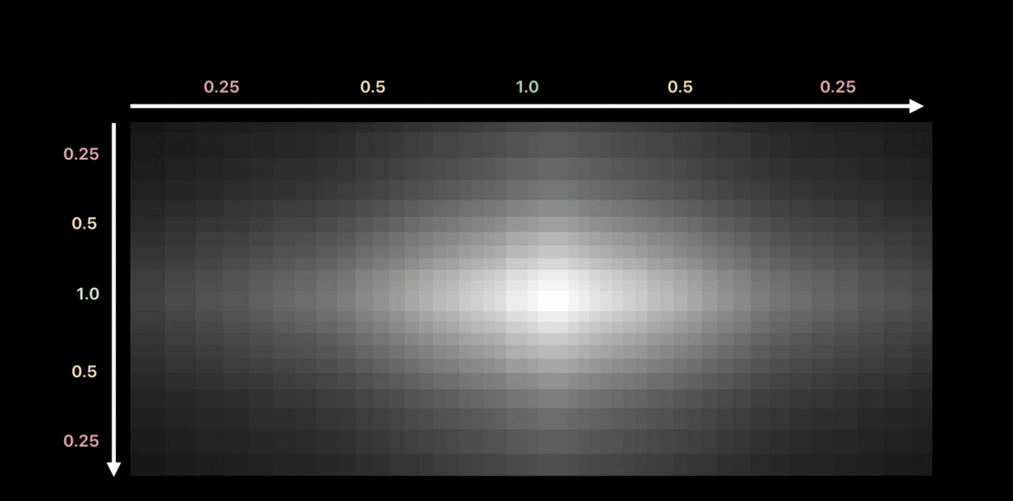
The mapping is defined as two 1D functions in the X and Y axes of the screen space.
You describe these functions in Metal using a series of control points defining the quality requirements.
In this image, we can see the effective rasterization rate across the screen, given our two 1D functions along the axis.
A quality level of one means that fragment shader is invoked for every screen space pixel along the axis.
And a quality level of 0.5 means that for at least 50 percent of the pixels, a fragment shader is invoked along a given axis.
A quality level of zero means that each fragment shader will be invoked at the minimum rate supported by Metal.
Metal will resample these control points to create a final rate map.
Even though you don’t control the final mapping directly, Metal guarantees that your minimum quality is preserved.
Now let’s create this mapping with Metal.
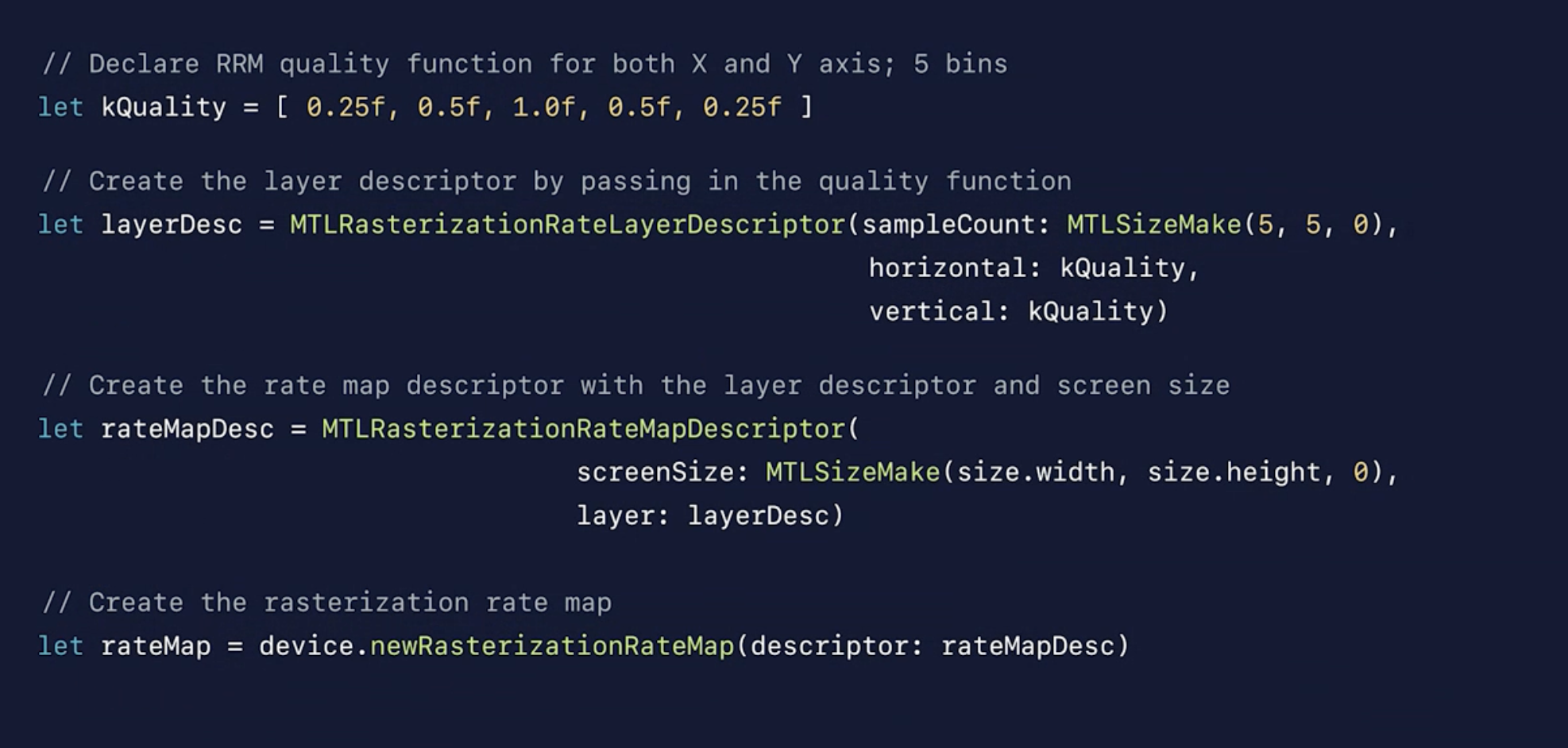
Here is the Metal code that builds the rasterization rate map you just saw.
First, you define the rasterization function.
In this example we will use the five values we showed previously for both the horizontal and vertical axis of our map.
You then fill the layer descriptor to describe the quality across our rasterization rate map.
You then create one by providing the horizontal and vertical quality functions.
With your quality defined, you now create a Metal rasterization rate map descriptor from the layer descriptor and our final screen space resolution.
Finally, you use your Metal device to instantiate a rasterization rate map object using that descriptor.
Next we need to create the physical render target for this map.
Because the actual rasterization rate map rates are implementation dependent, you need to first query the physical size of the resource from the map.
You then create the physical render target as usual: specify the correct usage and storage properties, and instantiate the texture using your Metal device object.
Finally, you combine the created texture and rasterization map to set up your render pass and render as usual.
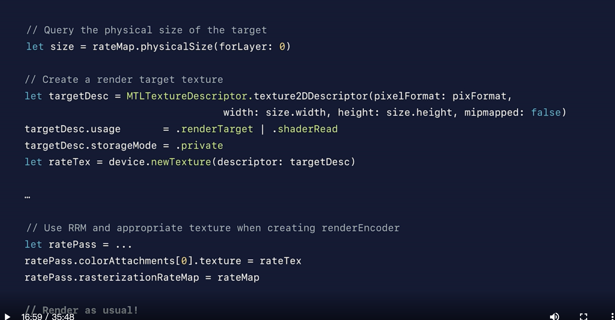
And with that, you have rasterized your g-buffer nonuniformly.

But what about shading the g-buffer in later passes? With a traditional deferred shading pipeline, you can continue lighting with the same rasterization rate map because your light geometry will get correctly rasterized in the same screen space as your g-buffer.

With tiled deferred renderers, you will need to do a little more work.
If you’re not already familiar with the tiled deferred rendering, please see our Modern Rendering with Metal talk at WWDC 2019.
With tiled deferred, your render target's physical space is split into equally sized blocks of pixels and each block performs light tile culling and shading.
In the presented image, our sample code shows a heat map for the number of lights per block of 32 by 32 pixels.
Because screen space no longer corresponds to physical space, integrating rasterization rate maps with tiled deferred renderers requires one additional step.
The lighting shader will need to transform the pixel coordinates in physical space to the virtual screen space.
This is the reverse mapping used during rasterization.
Let’s take a look at how you can perform this reverse mapping in your shaders.

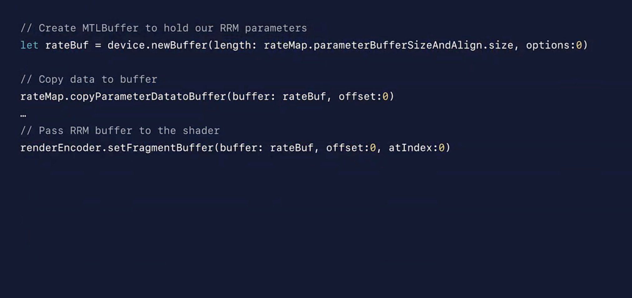
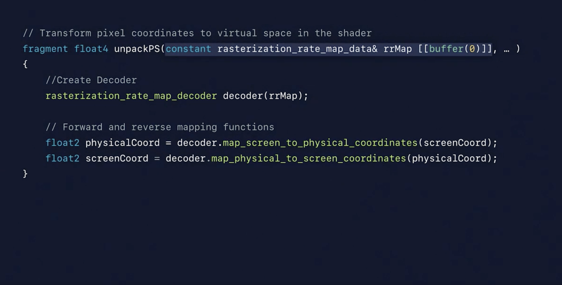
First you have to make the rasterization rate map parameters accessible to the shader.
To do this, first you create a MTLBuffer that can hold the parameters.
You then copy the parameter data into a MTLBuffer.
And finally, bind the MTLBuffer to your shader.
Now that the map is bound, let’s use it.
In the shader, you now have access to a rasterization_rate_map_data object at the corresponding buffer bind point.
You can use that object to instantiate a rasterization_rate_map_decoder object.
And then use the decoder to transform between the physical and screen coordinates.
Returning to our tiled deferred renderer, we use the decoder to perform tile culling in the virtual screen space.
Adapting your light culling to virtual screen space means your tiles are no longer square, but now follow the correct area in screen space.

Let’s compare this heat map to the full, uniform resolution render.

And back to the rasterization rate map version.
As you can see, with rasterization rate maps, we’ve significantly reduced the amount of shaded tiles on our screen.
Finally, let’s consider how rasterization rate maps are prepared for compositing and final presentation.
Before displaying the final image to the screen, you need to unwrap it using a full screen pass that transforms the physical space texture to a high-resolution surface using the shader mapping just described.


As you can see, it is very difficult to notice the quality trade-offs despite the aggressive falloffs that were chosen for this sample.
We expect rasterization rate maps to be combined with other techniques, such as depth of field, to hide the quality tradeoff.

That’s it for rasterization rate maps.
vertex amplification
Let’s move on to vertex amplification.
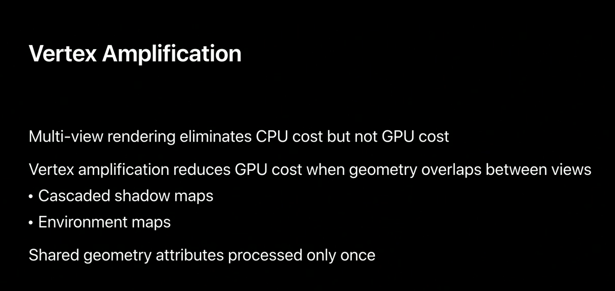
Vertex amplification lets you reduce geometry processing in multi-view rendering cases.

Multi-layer and multi-viewport rendering reduce the number of draw calls needed to target each view using instancing.
But that doesn’t eliminate the GPU cost of processing each of these instances.
Many multi-layer and multi-viewport rendering techniques share geometry between views.
For example, between the cascades of shadow maps or the sides of an environment map.
Each of those instances typically transform that geometry in almost the same way.
So even though the position is unique per view, attributes such as normals, tangents, and texture coordinates are identical.
Vertex amplification lets you process those shared attributes only once, increasing the efficiency of your vertex shading.
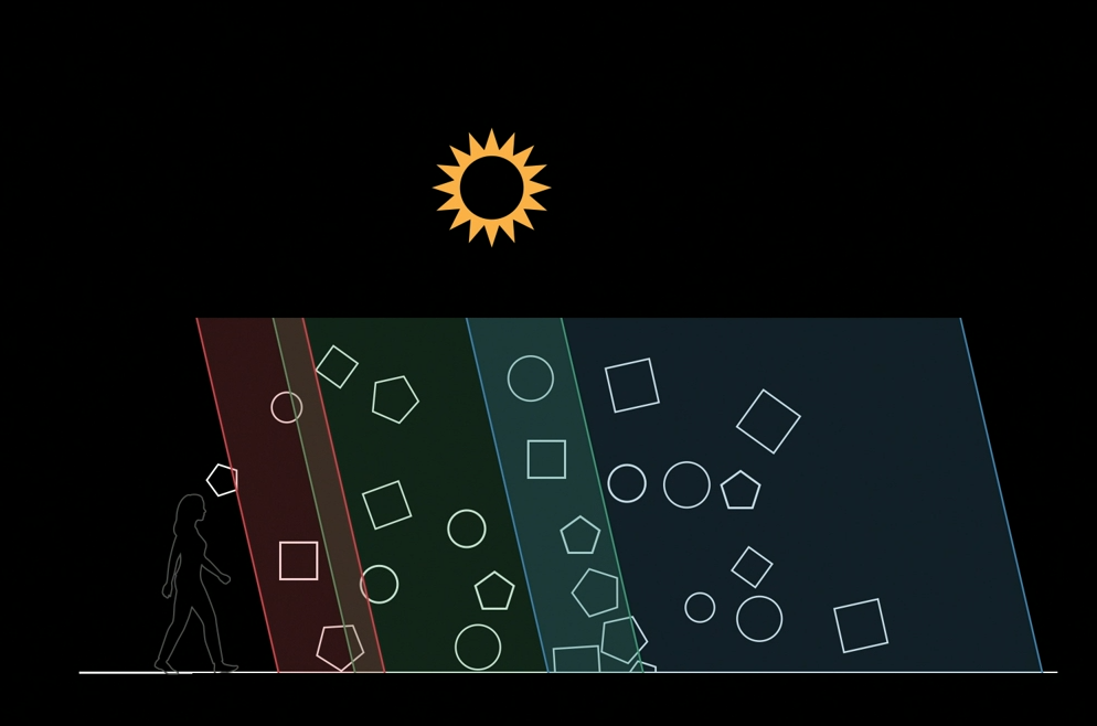
Let’s consider the use case of cascaded shadow maps in more detail.
Depending on the view distance, a renderer might split its shadow maps into one, two, or three or more overlapping shadow cascades.
As we increase the number of cascades, we also increase the size of the virtual world that each cascade covers.
This causes the larger, more distant cascades to accumulate more geometry in them, compared to closer cascades.
And with more cascades, the number of objects that render into more than one cascade increases.
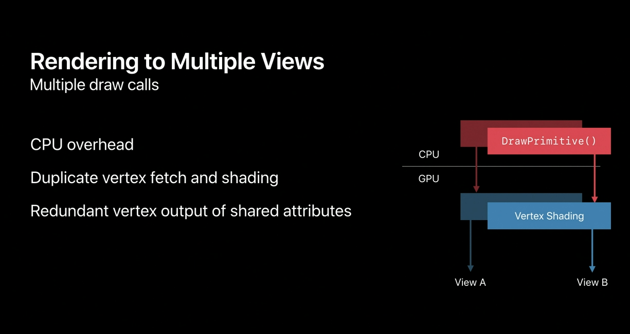
Now let’s consider how cascaded shadow maps are traditionally rendered and the associated costs.
Before multi-view rendering, you would simply draw into each cascade separately.
This increased both the GPU and CPU overhead.
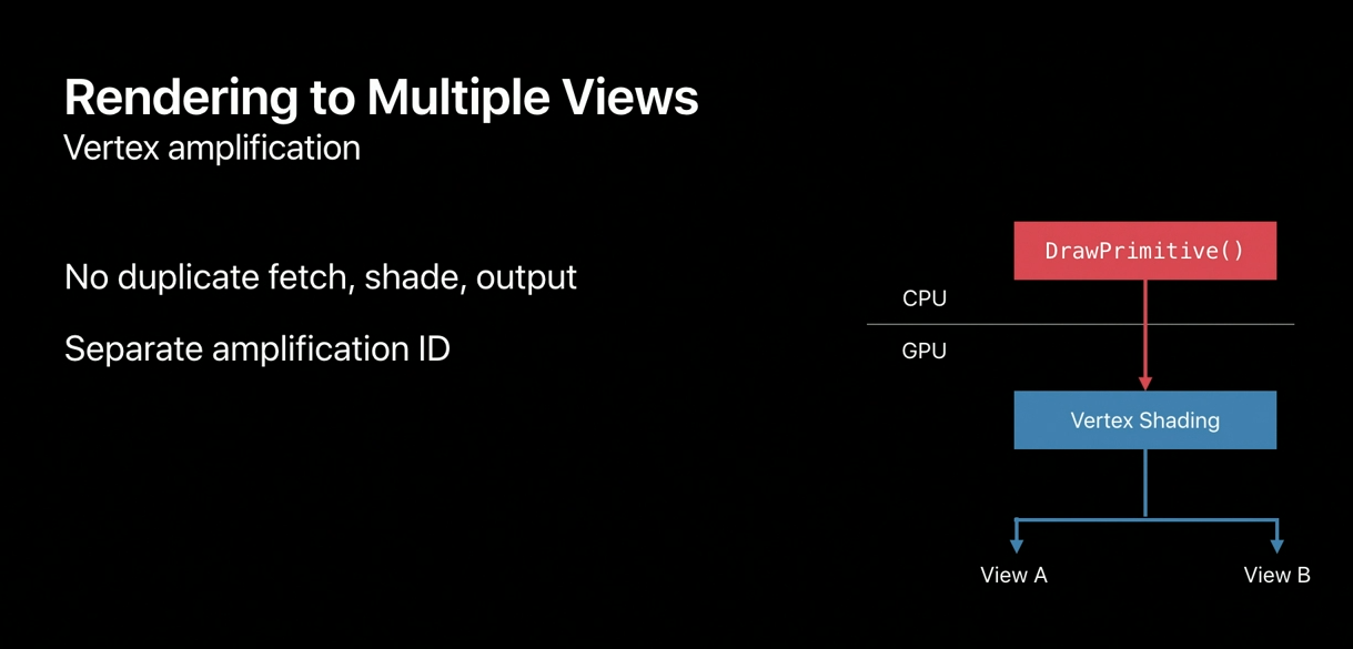
Each vertex must be fetched and shaded multiple times, and each vertex is also output multiple times.
Multi-view instance rendering uses the instance ID to map each primitive to its destination view.
It eliminates the CPU cost of multiple draw calls, but the GPU cost remains the same.
Using instancing for layered rendering also complicates rendering of actual instanced geometry, since instance ID now has to encode both the actual instance ID and the target layer.

Vertex amplification eliminates the duplicate fetch, shading, and output.
It also provides a separate amplification ID.
Let’s take a look at a vertex amplification in action.
Existing vertex functions can be easily adapted to vertex amplification.
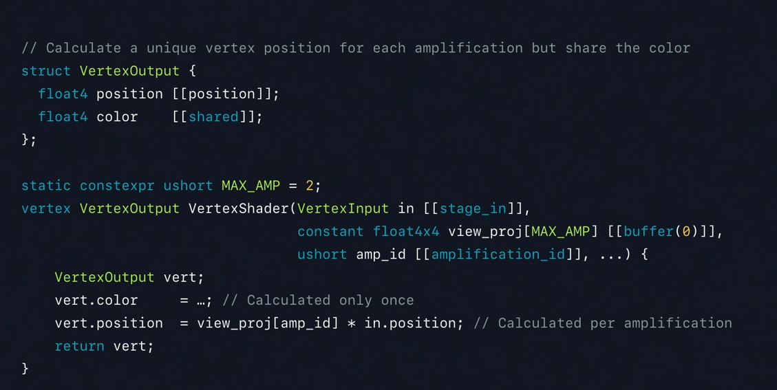
In this example, we’re going to calculate a unique position per amplification, but share the color calculation across all amplifications.
We start by declaring our VertexOutput with two attributes.
The compiler can usually infer if an attribute is unique or shared, but for complicated shaders, you can also be explicit about which attributes are shared.
The compiler will report an error when shared attribute calculations are dependent on amplification ID.
Next we declare a function argument holding the amplification ID.
Any calculations associated with this ID are amplified per shader invocation.
The color attribute is not associated with that ID so it will only be executed once.
But the position is dependent on the ID to look up the correct view projection matrix, and so the entire expression is amplified.
That’s it for the shader code.
Now let's see how we set up the amplified draw calls.
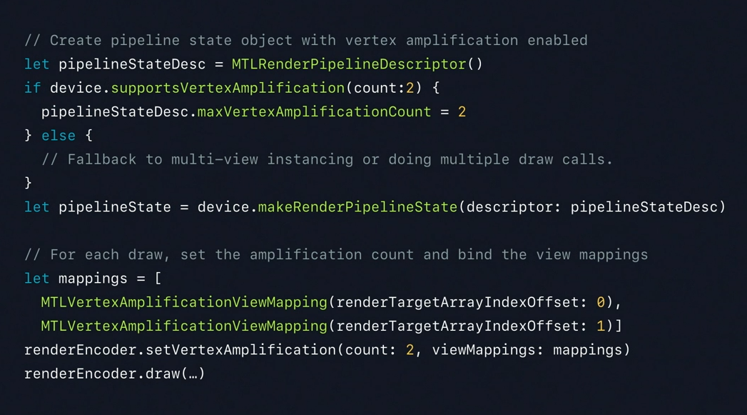
Let’s start by creating a pipeline state object that enables amplification.
The maximum amplification factor supported by Metal can be queried from the device.
In this case, let’s say you want an amplification factor of two.
If supported, you set to maximum amplification factor for the pipeline.
If not supported, you can fall back to traditional multi-view through instancing or rely on doing multiple draw calls.
Finally, you create the pipeline.
Once the pipeline is created, and assuming that amplification is supported, you can start to encode your draws.
Drawing with amplification requires setting the amplification count and binding the viewMappings.
viewMappings describe how to map the amplification ID to target layer or viewport.
If the vertex shader also exports a render target or viewport array index, that index will serve as a base offset into the viewMappings array.
Now you can set the desired amplification and encode the draws.
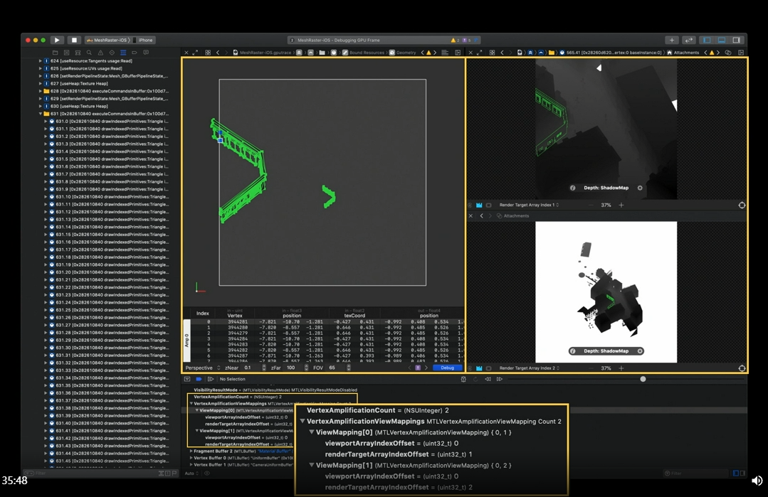
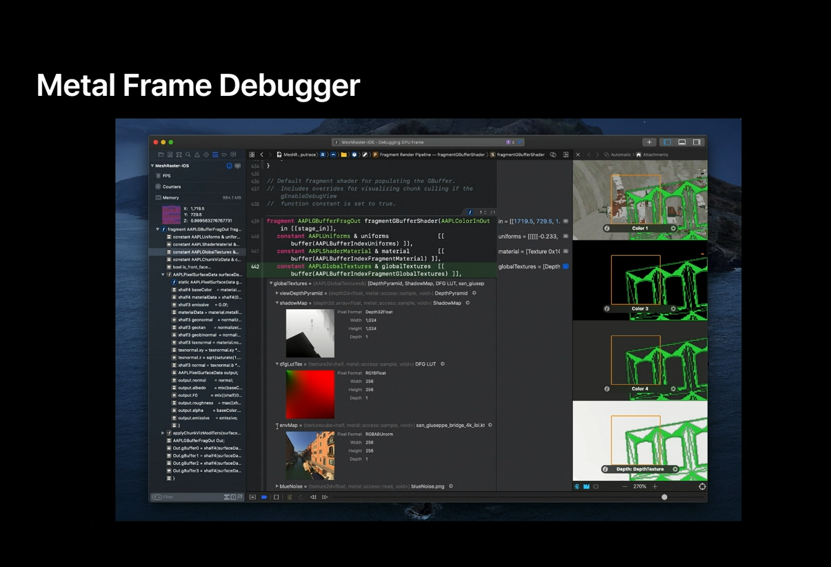
Let’s take a closer look through the Metal frame debugger.
In this sample render, we use VertexAmplification to amplify all the draws that are rendered to both cascades 2 and 3.
Here we see that this draw call is rendered with a ViewMapping that specifies two render targets.
The mesh is rendered simultaneously into the second cascade shown on the left, and the third cascade, shown both on the right and in the geometry viewer.
That’s it for vertex amplification.
argument buffers
Let’s move on to argument buffers and how they’ve been extended for the A13.
We introduced argument buffers with Metal 2.
Argument buffers allow you to encode constants, textures, samplers, and buffer arguments into MTLBuffers.
By encoding all your draw arguments into a single Metal argument buffer, you can render complex scenes with minimal CPU overhead.
Once encoded, you can reuse argument buffers to avoid repeated redundant resource binding.
Argument buffers are also necessary to enable GPU-driven pipelines, by providing access to the entire scene’s draw arguments on the GPU.
You can then modify argument buffers in compute functions to dynamically configure your scene, just in time.

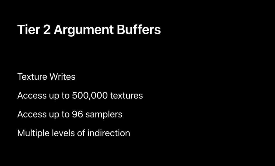
Tier 2 argument buffers dramatically enhance the capabilities of argument buffers.
With A13, your Metal functions can sample or write to any texture in an argument buffer.
You can also access a virtually unlimited number of textures and many samplers.
And argument buffers can now also reference other argument buffers with multiple levels of indirection.
This unlocks the ability to encode a single argument buffer for all your scene data and access it in your draw without needing to assemble argument buffers ahead of time on GPU or CPU.
Let’s look at an example.
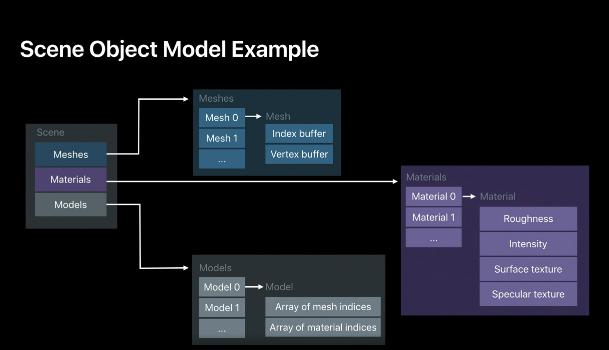
Here is an example scene object model hierarchy.
We showed a similar example at our Modern Rendering with Metal talk at WWDC 2019.
The hierarchy describes all your geometry data, materials, and model data.
With argument buffers, we can encode this object model directly.
But with Tier 2 support we can also use the hierarchy directly during rendering.
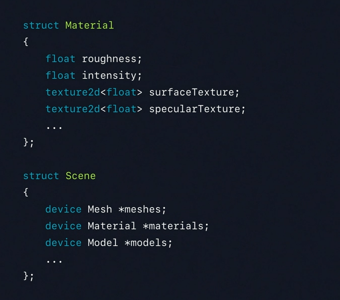
Let’s take a look at an example shader.
To start, recall that our argument buffers are declared in the Metal shading language as structures of constants, textures, samplers, and buffers.
These declarations directly mirror the example object hierarchy just described.
The first is our material representation, and the second is our scene that references the set of meshes, materials, and models.
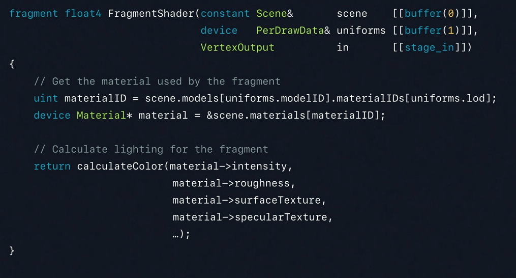
OK, so now let’s take a look at a fragment function that shades using our scene directly.
The first function parameter is our scene argument buffer.
The second function parameter is our per-draw constants.
In this example, it encodes the model ID for this draw, as well as the discrete level of detail, both chosen in an earlier compute pass.
We then use these IDs to fetch our material from the scene using the IDs computed earlier.
And we calculate the fragment color using the textures, constants, and samplers from the nested argument buffer.
And that’s it! No more intervening compute pass to gather material parameters into per-draw argument buffers.
The fragment shader just uses the scene argument buffer directly.
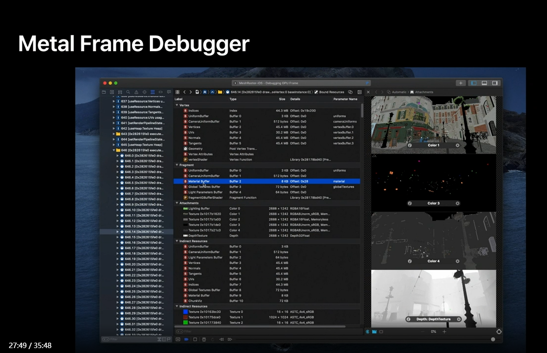
Before we move on though, I’d like to highlight the robust tool support for argument buffers.
With argument buffers and GPU-driven pipelines, your scene setup moves to the GPU, and so does any debugging.
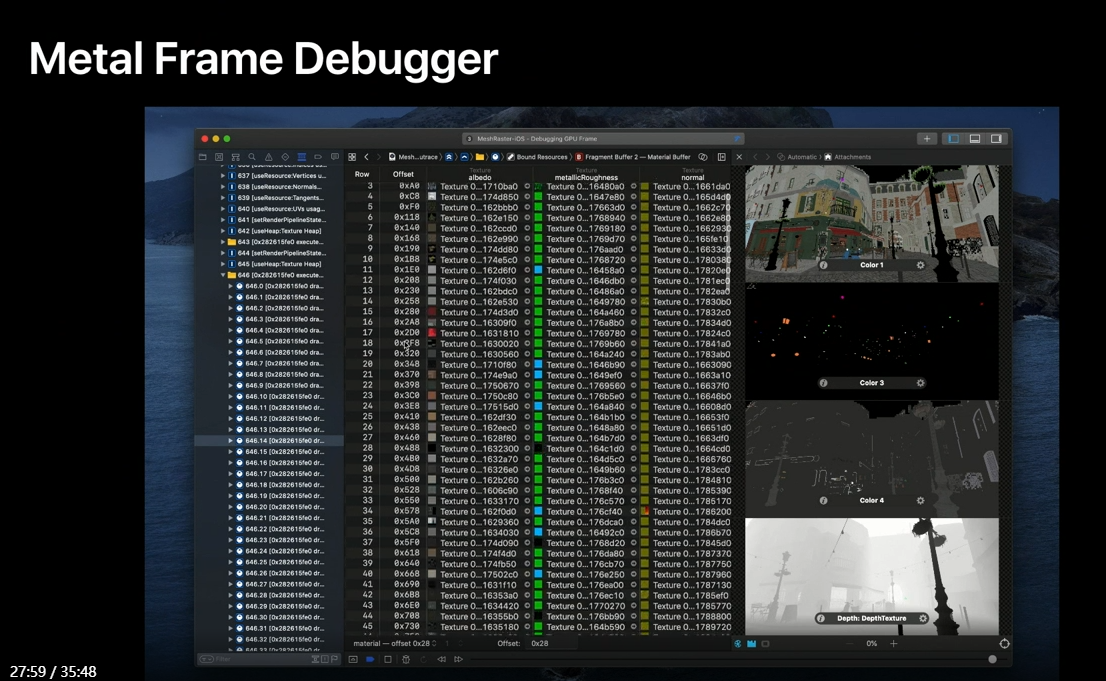
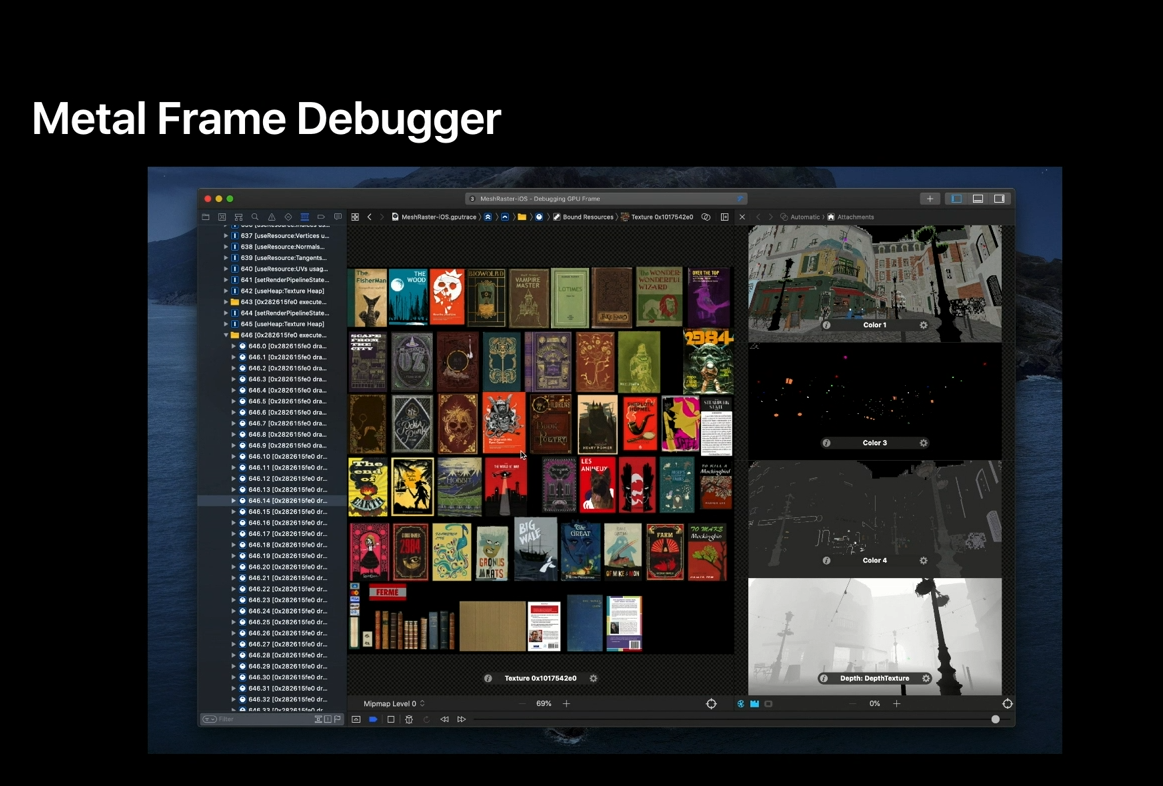
The Metal frame debugger allows you to easily debug and inspect both argument buffers and the shaders that use them.
You can use the buffer viewer to inspect all resources in your argument buffer, and quickly jump to these resources for further inspection.
You can also use the shader debugger to understand how your shaders are accessing or building argument buffers.
This is especially important when calculating argument buffer indices or modifying argument buffers on the GPU.
That's it for Tier 2 argument buffers.
simd
Now let’s move on to a new class of shader optimization techniques.
SIMD group functions are a powerful tool for optimizing compute and graphics functions.
They allow a GPU workload to share data and control flow information by leveraging the architecture of the GPU.
Let's unpack that by quickly reviewing the SIMD execution model in Metal.

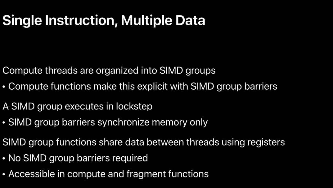
Metal has always organized threads into SIMD groups to exploit the single Instruction, multiple data nature of GPUs.
You may have leveraged SIMD groups in Metal compute functions to reduce the costs of synchronizing entire threadgroups by using SIMD group barriers instead.
The threads of a SIMD group execute in lockstep, so execution barriers are not needed.
A SIMD group barrier therefore only synchronizes memory operations.
SIMD group functions exploit this lockstep execution to share data between its threads using registers instead of threadgroup memory, and can significantly improve performance when threadgroup memory bound.
They’re also available for both compute and render functions.
And as we’ll see in a bit, this enables a very interesting render optimization technique.
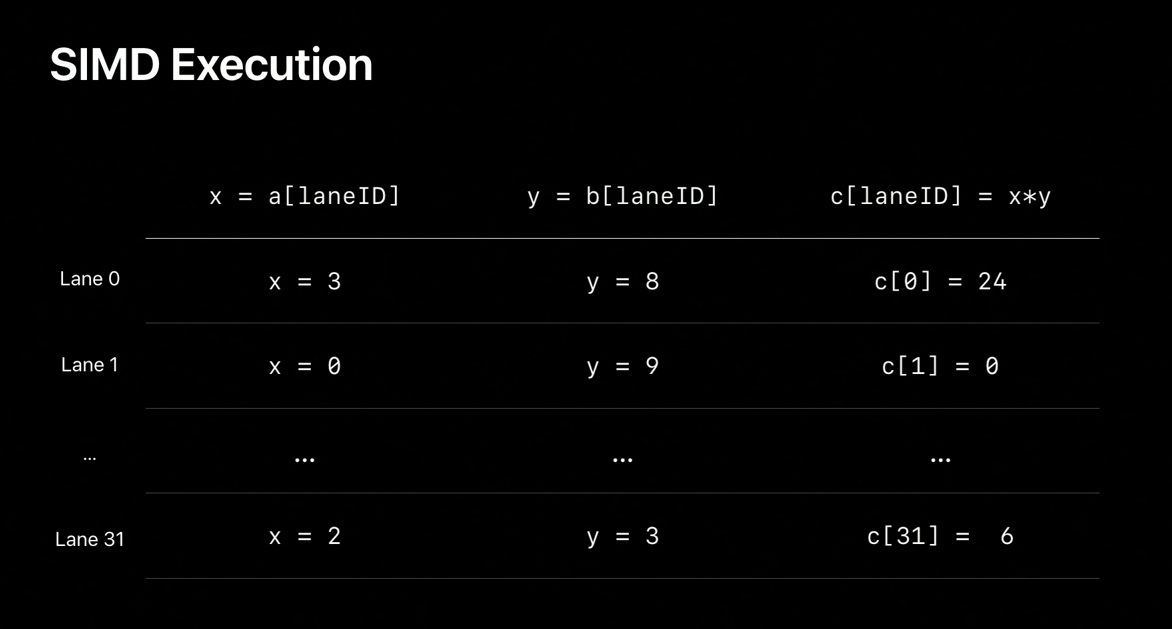
Let’s first start by building a better intuition for SIMD execution with an example.
Down the left side we represent a SIMD group as 32 lanes starting with Lane 0.
A lane is a single thread in a SIMD group.
Now let’s make this SIMD group perform some work.
First we have all lanes index an array, A, by its laneID and store the result in a variable X.
Note how each lane has its own value of X.
In this execution model, the instruction to load the data from A is only fetched once and executed simultaneously by 32 threads that have their own indices.
Now we read a second array, B, indexed by laneID and store the result in Y.
Finally we store the result of multiplying X and Y in a third array, C.
Since the instruction executed is only fetched once for the whole group, all SIMD group threads execute in lockstep.
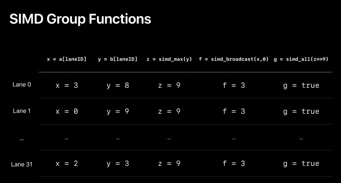
SIMD group functions allow each thread in the group to inspect register values of the entire SIMD group with minimal overhead.
This ability allows for some interesting functions.
First let’s introduce simd_max and apply it to variable Y.
Each thread gets a Z value with the largest value from Y, as seen by any thread in the SIMD group.
Next we have broadcast and apply it to X.
In this example, we broadcast the value of Lane 0 to all the other lanes in a single operation.
Metal for A13 supports many other similarly operating SIMD functions such as shuffle, permute, and rotate across all lanes.
For our final example we’ll take a look at simd_all, which tells each lane whether an expression evaluates the same for all lanes.
In this example the Z variable is indeed nine for all lanes, and we therefore return true.
Likewise, simd_any tells whether an expression evaluates to true for any lane.
You can use simd_all to reduce divergence in your shaders by choosing to take a more optimal path when all threads have the same need.
Let’s take a look at an example.
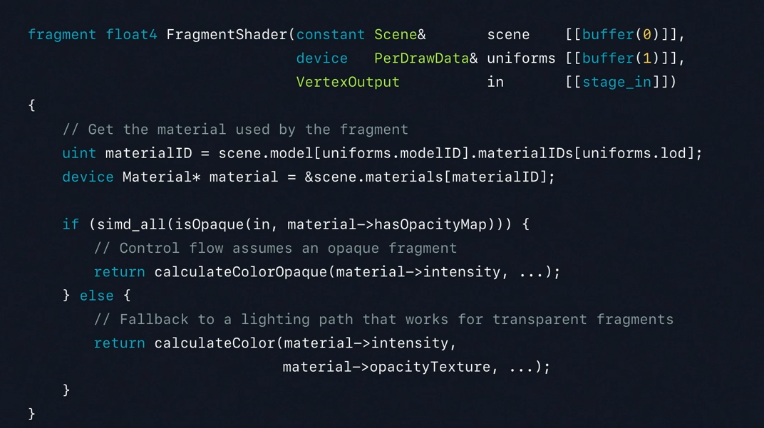
Here is our fragment shader from earlier with some optimizations using SIMD group functions.
To recap, this function takes as inputs the scene encoded as an argument buffer, uniforms, and the vertex stage_in.
Typically, lighting functions evaluate various components of the final color differently for transparent fragments and thus require dynamic control flow at various points.
Now, instead of evaluating the opacity for every fragment, here we use simd_all to check dynamically if all the threads in the SIMD group are computing the lighting for opaque fragments.
If they are, we take an optimal path that assumes only opaque objects.
And if not, we fall back to the earlier path that can light both opaque and transparent fragments.
That’s it for SIMD group functions on A13.
astc hdr
Let’s switch gears and look at some of the exciting additions to ASTC on A13.
As mentioned earlier in the video, the A13 GPU doubles the rate of 16-bit floating point operations and adds support for small 16-bit numbers to better handle HDR processing.
Apps take advantage of these improvements without any modification; HDR processing on the GPU just gets faster and more accurate.
Apple Family 6 also adds support for a new set of pixel formats that support the efficient storage and sampling of HDR data called ASTC HDR.
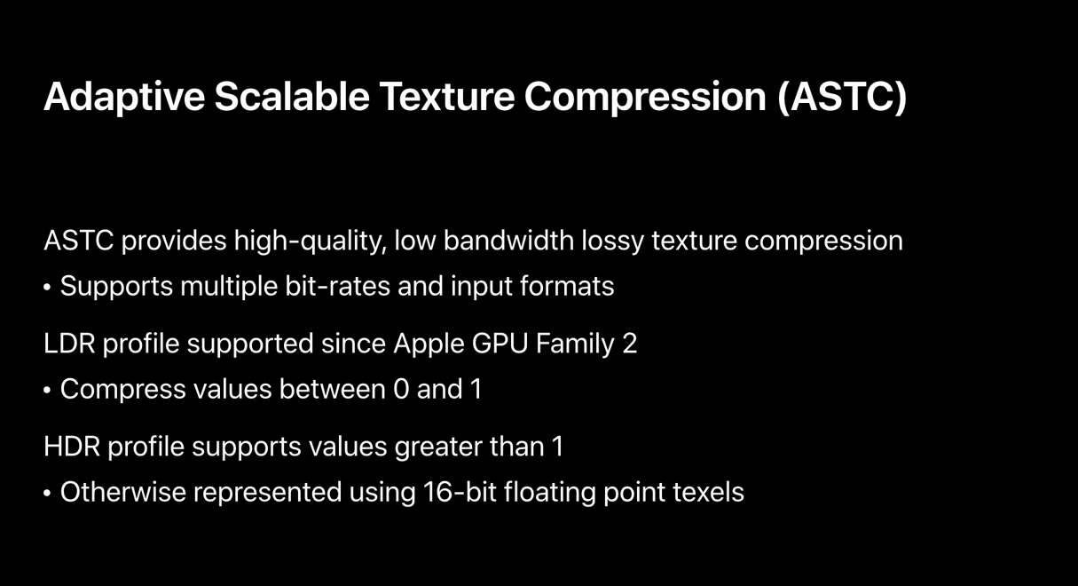
ASTC is a texture compression technology supported on many platforms, providing high texture image quality at a fraction of the bandwidth and memory.
It does so by supporting multiple bit rates and input formats.
The ASTC low dynamic range profile has been supported since Apple GPU Family 2 and is appropriate for compressing values in the zero to one range.
If your app is not already using ASTC to save memory and bandwidth, we highly encourage you to do so.
The high dynamic range profile is needed to encode the larger brightness values found in HDR images.
Without ASTC HDR, such images are typically stored in 16-bit floating point pixel formats at much higher memory cost.
So how much storage can ASTC HDR save? A lot.
Let’s consider an example.
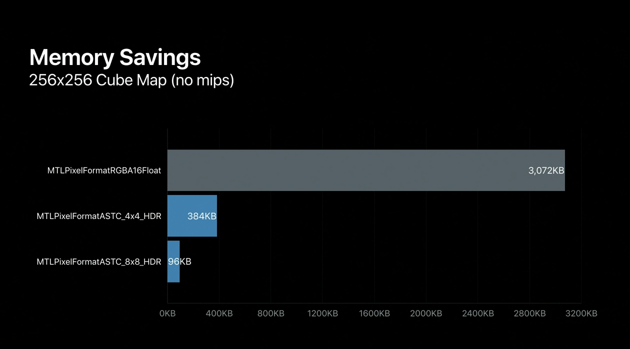
HDR games often use low-resolution cube map textures to represent high dynamic range environment maps to light their scene, and typically place many such probes across the game world or level.
Without ASTC HDR, each probe can consume a significant amount of memory, and all such probes can easily consume a large portion of your game’s memory budget.
In this example, a 256 by 256 probe cube map alone consumes 3MB.
With ASTC HDR, the same probe would consume many times less memory.
You can even vary the bit rate to really reduce the footprint.
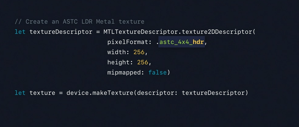
Creating an HDR texture is as simple as an LDR equivalent.
In this example, we’re creating a four by four ASTC LDR texture.
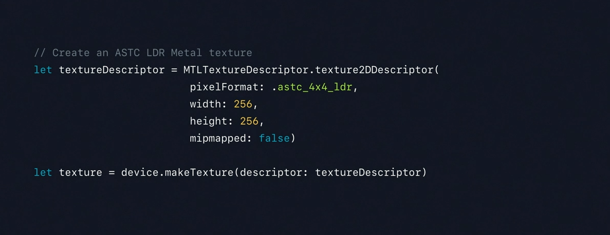
There is matching HDR format for every LDR format so converting this to an HDR texture just requires changing the pixel format.
All right, that wraps up the new Metal features for the A13 GPU.
Let’s recap what we’ve learned.
It enables higher quality texture streaming with sparse textures.
It lets you focus expensive shading to where needed with rasterization rate maps, and eliminate redundant vertex processing with vertex amplification.
It also enables more flexible GPU-driven pipelines with argument buffer Tier 2, and SIMD group sharing with shuffle and ballot instructions.
And finally, Metal now lets you save memory in HDR pipelines with ASTC.
For more information about Metal, the A13 GPU, and to find our latest sample code, please visit developer.apple.com. Thank you.
虽然并非全部原创,但还是希望转载请注明出处:电子设备中的画家|王烁 于 2022 年 5 月 25 日发表,原文链接(http://geekfaner.com/shineengine/WWDC2020_MetalEnhancementsforA13Bionic.html)